Rolling forecasts
Alexander Häußer
Source:vignettes/vignette_202_tidy_m4_monthly_splits.Rmd
vignette_202_tidy_m4_monthly_splits.RmdIntroduction
This vignette demonstrates how to evaluate Echo State Network
forecasts across multiple rolling windows using the tidy interface of
echos. Rolling forecast evaluation provides a more robust
assessment than a single train-test split because the model is estimated
and evaluated at several forecast origins.
The example uses two monthly time series from
m4_monthly_subset. Fixed training windows are created with
slide_tsibble() from the tsibble package. For
every series and split, an ESN is fitted and used to generate an
18-month-ahead forecast.
Prepare the data
The dataset is filtered to the two time series "M21655"
and "M2717".
selected_series <- c("M21655", "M2717")

data_frame <- m4_monthly_subset %>%
  filter(series %in% selected_series)

data_frame
#> # A tsibble: 494 x 4 [1M]
#> # Key:       series [2]
#>    series category       index value
#>    <chr>  <fct>          <mth> <dbl>
#>  1 M21655 Demographic 1995 Jan  4970
#>  2 M21655 Demographic 1995 Feb  5010
#>  3 M21655 Demographic 1995 Mar  5060
#>  4 M21655 Demographic 1995 Apr  5010
#>  5 M21655 Demographic 1995 May  5610
#>  6 M21655 Demographic 1995 Jun  6040
#>  7 M21655 Demographic 1995 Jul  6450
#>  8 M21655 Demographic 1995 Aug  6370
#>  9 M21655 Demographic 1995 Sep  5190
#> 10 M21655 Demographic 1995 Oct  5250
#> # ℹ 484 more rows
p <- ggplot()

p <- p + geom_line(
  data = data_frame,
  aes(
    x = index,
    y = value),
  linewidth = 0.5
)

p <- p + facet_wrap(
  vars(series),
  ncol = 1,
  scales = "free_y"
)

p <- p + labs(
  x = "Time",
  y = "Value"
)

p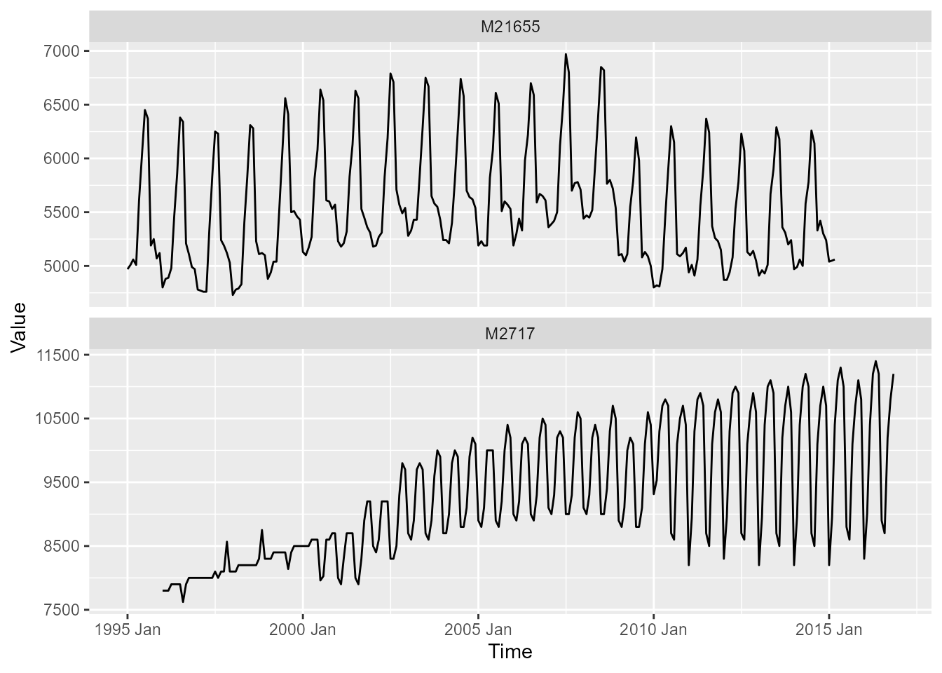
Define the rolling forecast setup
Each ESN is trained on a fixed window of 180 monthly observations. The forecast horizon is 18 months, corresponding to the horizon used for monthly series in the M4 Forecasting Competition. The forecast origin advances by one month between splits.
Five splits are used in this example. To reduce the vignette runtime,
set n_splits to a smaller value such as 3.
n_train <- 180
n_ahead <- 18
n_step <- 1
n_splits <- 5

n_required <- n_train + n_ahead + (n_splits - 1) * n_step
Only the most recent observations required for the rolling evaluation are retained. This ensures that both series contribute the same number of observations and splits.
analysis_frame <- data_frame %>%
  group_by_key() %>%
  slice_tail(n = n_required) %>%
  ungroup()

analysis_frame
#> # A tsibble: 404 x 4 [1M]
#> # Key:       series [2]
#>    series category       index value
#>    <chr>  <fct>          <mth> <dbl>
#>  1 M21655 Demographic 1998 Jun  5830
#>  2 M21655 Demographic 1998 Jul  6310
#>  3 M21655 Demographic 1998 Aug  6280
#>  4 M21655 Demographic 1998 Sep  5230
#>  5 M21655 Demographic 1998 Oct  5110
#>  6 M21655 Demographic 1998 Nov  5120
#>  7 M21655 Demographic 1998 Dec  5100
#>  8 M21655 Demographic 1999 Jan  4880
#>  9 M21655 Demographic 1999 Feb  4940
#> 10 M21655 Demographic 1999 Mar  5040
#> # ℹ 394 more rows
Create rolling training windows
slide_tsibble() creates fixed rolling windows by
observation. The new variable split is added to the tsibble
key and identifies the individual training windows.
train_frame <- analysis_frame %>%
  slide_tsibble(
    .size = n_train,
    .step = n_step,
    .id = "split"
  ) %>%
  filter(split <= n_splits)

train_frame
#> # A tsibble: 1,800 x 5 [1M]
#> # Key:       split, series [10]
#>    series category       index value split
#>    <chr>  <fct>          <mth> <dbl> <int>
#>  1 M21655 Demographic 1998 Jun  5830     1
#>  2 M21655 Demographic 1998 Jul  6310     1
#>  3 M21655 Demographic 1998 Aug  6280     1
#>  4 M21655 Demographic 1998 Sep  5230     1
#>  5 M21655 Demographic 1998 Oct  5110     1
#>  6 M21655 Demographic 1998 Nov  5120     1
#>  7 M21655 Demographic 1998 Dec  5100     1
#>  8 M21655 Demographic 1999 Jan  4880     1
#>  9 M21655 Demographic 1999 Feb  4940     1
#> 10 M21655 Demographic 1999 Mar  5040     1
#> # ℹ 1,790 more rows
The following summary shows the start and end of every training window.
split_frame <- train_frame %>%
  as_tibble() %>%
  summarise(
    train_start = min(index),
    train_end = max(index),
    n = n(),
    .by = c(series, split)
  )

split_frame
#> # A tibble: 10 × 5
#>    series split train_start train_end     n
#>    <chr>  <int>       <mth>     <mth> <int>
#>  1 M21655     1    1998 Jun  2013 May   180
#>  2 M2717      1    2000 Feb  2015 Jan   180
#>  3 M21655     2    1998 Jul  2013 Jun   180
#>  4 M2717      2    2000 Mar  2015 Feb   180
#>  5 M21655     3    1998 Aug  2013 Jul   180
#>  6 M2717      3    2000 Apr  2015 Mar   180
#>  7 M21655     4    1998 Sep  2013 Aug   180
#>  8 M2717      4    2000 May  2015 Apr   180
#>  9 M21655     5    1998 Oct  2013 Sep   180
#> 10 M2717      5    2000 Jun  2015 May   180
Train the ESN models
The combination of series and split forms
the key of train_frame. Consequently, model()
estimates one ESN for each series and rolling window. With two series
and five splits, ten ESN models are trained.
Because the ESN reservoir is initialized randomly, a seed is set to make the results reproducible.
model_frame <- train_frame %>%
  model(
    "ESN" = ESN(value)
  )

model_frame
#> # A mable: 10 x 3
#> # Key:     split, series [10]
#>    split series                             ESN
#>    <int> <chr>                          <model>
#>  1     1 M21655  <ESN({72, 1, 1}, {144, 17.7})>
#>  2     1 M2717  <ESN({72, 1, 1}, {144, 25.29})>
#>  3     2 M21655 <ESN({72, 1, 1}, {144, 16.78})>
#>  4     2 M2717   <ESN({72, 1, 1}, {144, 25.4})>
#>  5     3 M21655 <ESN({72, 1, 1}, {144, 18.05})>
#>  6     3 M2717   <ESN({72, 1, 1}, {144, 25.3})>
#>  7     4 M21655 <ESN({72, 1, 1}, {144, 16.01})>
#>  8     4 M2717  <ESN({72, 1, 1}, {144, 25.25})>
#>  9     5 M21655  <ESN({72, 1, 1}, {144, 25.7})>
#> 10     5 M2717  <ESN({72, 1, 1}, {144, 25.11})>
Generate rolling forecasts
An 18-month-ahead forecast is generated for each fitted ESN.
fable_frame <- model_frame %>%
  forecast(h = n_ahead)

fable_frame
#> # A fable: 180 x 6 [1M]
#> # Key:     split, series, .model [10]
#>    split series .model    index
#>    <int> <chr>  <chr>     <mth>
#>  1     1 M21655 ESN    2013 Jun
#>  2     1 M21655 ESN    2013 Jul
#>  3     1 M21655 ESN    2013 Aug
#>  4     1 M21655 ESN    2013 Sep
#>  5     1 M21655 ESN    2013 Oct
#>  6     1 M21655 ESN    2013 Nov
#>  7     1 M21655 ESN    2013 Dec
#>  8     1 M21655 ESN    2014 Jan
#>  9     1 M21655 ESN    2014 Feb
#> 10     1 M21655 ESN    2014 Mar
#> # ℹ 170 more rows
#> # ℹ 2 more variables: value <dist>, .mean <dbl>
Evaluate forecast accuracy
The forecasts are evaluated against the corresponding observations in
analysis_frame. Accuracy measures are calculated separately
for every series and split.
accuracy_frame <- fable_frame %>%
  accuracy(data = analysis_frame)

accuracy_frame
#> # A tibble: 2 × 11
#>   .model series .type    ME  RMSE   MAE    MPE  MAPE  MASE RMSSE    ACF1
#>   <chr>  <chr>  <chr> <dbl> <dbl> <dbl>  <dbl> <dbl> <dbl> <dbl>   <dbl>
#> 1 ESN    M21655 Test  -74.0  116.  94.4 -1.41   1.78 0.667 0.580 -0.0121
#> 2 ESN    M2717  Test  -59.3  250. 214.  -0.660  2.12 1.19  0.911  0.753
Visualize the rolling forecasts
For each series and split, the point forecasts are compared with the observed values over the 18-month evaluation period.
forecast_frame <- fable_frame %>%
  as_tibble() %>%
  transmute(
    series,
    split,
    index,
    FORECAST = .mean
  )

plot_frame <- forecast_frame %>%
  left_join(
    analysis_frame %>%
      as_tibble() %>%
      select(
        series,
        index,
        ACTUAL = value),
    by = c(
      "series",
      "index")) %>%
  pivot_longer(
    cols = c(ACTUAL, FORECAST),
    names_to = "type",
    values_to = "value"
    )

plot_frame
#> # A tibble: 360 × 5
#>    series split    index type     value
#>    <chr>  <int>    <mth> <chr>    <dbl>
#>  1 M21655     1 2013 Jun ACTUAL   5900
#>  2 M21655     1 2013 Jun FORECAST 5962.
#>  3 M21655     1 2013 Jul ACTUAL   6290
#>  4 M21655     1 2013 Jul FORECAST 6327.
#>  5 M21655     1 2013 Aug ACTUAL   6180
#>  6 M21655     1 2013 Aug FORECAST 6150.
#>  7 M21655     1 2013 Sep ACTUAL   5360
#>  8 M21655     1 2013 Sep FORECAST 5480.
#>  9 M21655     1 2013 Oct ACTUAL   5310
#> 10 M21655     1 2013 Oct FORECAST 5397.
#> # ℹ 350 more rows
p <- ggplot()

p <- p + geom_line(
  data = plot_frame,
  aes(
    x = index,
    y = value,
    color = type),
  linewidth = 0.6
)

p <- p + facet_grid(
  rows = vars(series),
  cols = vars(split),
  scales = "free_y"
)

p <- p + scale_color_manual(
  values = c(
    "ACTUAL" = "grey35",
    "FORECAST" = "steelblue"
  )
)

p <- p + labs(
  title = "Rolling forecasts for M4 monthly time series",
  subtitle = "Fixed 180-month training windows and an 18-month forecast horizon",
  x = "Time",
  y = "Value",
  color = NULL
)

p <- p + theme(legend.position = "top")

p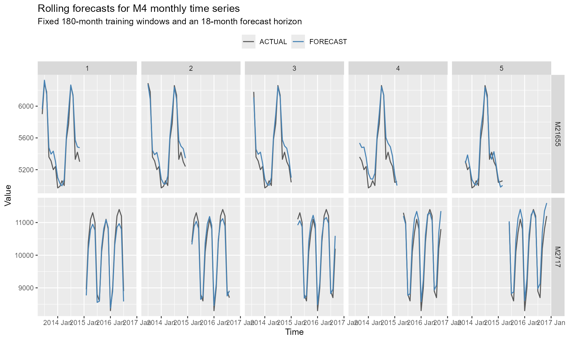
Summary
This example combines the tidy interface of echos with
rolling-window functionality from tsibble. The workflow
consists of four main steps:
- Create multiple fixed training windows with
slide_tsibble(). - Estimate one ESN for each series and split with
model(). - Generate forecasts with
forecast(). - Evaluate the forecasts across splits with
accuracy().
The same workflow can be extended to more series, additional forecast
origins, or alternative models supported by the fable
framework.