Prepare dataset
In a first example, we want to model the well-known
AirPassengers time series (ts object). The
dataset contains monthly totals of international airline passengers (in
thousands) from January 1949 to December 1960 with 144 observations in
total. The first 132 observations are used for model training
(n_train) and the last 12 observations are used for testing
(n_ahead). xtrain and xtest are
numeric vectors containing the training and testing data.
# Convert 'AirPassengers' dataset from ts to numeric vector
xdata <- as.numeric(AirPassengers)
# Forecast horizon
n_ahead <- 12
# Number of observations (total)
n_obs <- length(xdata)
# Number of observations (training data)
n_train <- n_obs - n_ahead

# Prepare train and test data
xtrain <- xdata[(1:n_train)]
xtest <- xdata[((n_train+1):n_obs)]

xtrain
#>   [1] 112 118 132 129 121 135 148 148 136 119 104 118 115 126 141 135 125 149
#>  [19] 170 170 158 133 114 140 145 150 178 163 172 178 199 199 184 162 146 166
#>  [37] 171 180 193 181 183 218 230 242 209 191 172 194 196 196 236 235 229 243
#>  [55] 264 272 237 211 180 201 204 188 235 227 234 264 302 293 259 229 203 229
#>  [73] 242 233 267 269 270 315 364 347 312 274 237 278 284 277 317 313 318 374
#>  [91] 413 405 355 306 271 306 315 301 356 348 355 422 465 467 404 347 305 336
#> [109] 340 318 362 348 363 435 491 505 404 359 310 337 360 342 406 396 420 472
#> [127] 548 559 463 407 362 405
xtest
#>  [1] 417 391 419 461 472 535 622 606 508 461 390 432
ESN architecture and automatic model selection
An Echo State Network consists of an input layer, a recurrent
reservoir, and a readout layer. In echos, the input and
reservoir weight matrices are randomly initialized and kept fixed. Only
the readout layer is estimated, using ridge regression.
The main reservoir hyperparameters are n_states,
alpha, rho, and density. The
argument n_states controls the reservoir size. The leakage
rate alpha controls how quickly reservoir states react to
new inputs. The spectral radius rho scales the recurrent
reservoir matrix and affects memory and stability. The argument
density controls the sparsity of the reservoir matrix.
The function train_esn() also performs automatic model
selection for the ridge readout. If n_models = NULL, the
function evaluates n_states * 2 candidate readout models.
Candidate ridge penalties are sampled from the interval specified by
lambda, and the best readout model is selected using the
information criterion specified by inf_crit.
Train ESN model
The function train_esn() is used to automatically train
an ESN to the input data xtrain, where the output
xmodel is an object of class esn. The object
xmodel is a list containing the actual and
fitted values, residuals, the internal states
states_train, estimated coefficients from the ridge
regression estimation, hyperparameters, etc. We can summarize the model
by using the generic S3 method summary() to get detailed
information on the trained model.
# Train ESN model
xmodel <- train_esn(y = xtrain)

# Summarize model
summary(xmodel)
#>
#> --- Inputs -----------------------------------------------------
#> n_obs        = 132
#> n_diff       = 1
#> lags         = 1
#>
#> --- Reservoir generation ---------------------------------------
#> n_states     = 52
#> alpha        = 1
#> rho          = 1
#> density      = 0.5
#> scale_inputs = [-0.5, 0.5]
#> scale_win    = [-0.5, 0.5]
#> scale_wres   = [-0.5, 0.5]
#>
#> --- Model selection --------------------------------------------
#> n_models     = 104
#> df           = 15.53
#> lambda       = 0.036
From the output above, we get the following information about the trained ESN model:
| Value | Description |
|---|---|
n_obs |
Number of observations (i.e., length of the input time series) |
n_diff |
Number of differences required to achieve (weak-) stationarity of the input training data |
lags |
Lags of the output variable (response), which are used as model input |
n_states |
Number of internal states (i.e., predictor variables or reservoir size). |
alpha |
Leakage rate (smoothing parameter) |
rho |
Spectral radius for scaling the reservoir weight matrix |
density |
Density of the reservoir weight matrix |
scale_inputs |
Input training data are scaled to the interval
(-0.5, 0.5)
|
scale_win |
Input weight matrix is drawn from a random uniform
distribution on (-0.5, 0.5)
|
scale_wres |
Reservoir weight matrix is drawn from a random uniform
distribution on (-0.5, 0.5)
|
n_models |
Number of models evaluated during the random search
optimization to find the regularization parameter
lambda
|
df |
Effective degrees of freedom in the model |
lambda |
Regularization parameter for the ridge regression estimation |
Forecast ESN model
The function forecast_esn() is used to forecast the
trained model xmodel for n_ahead steps into
the future. The output xfcst is a list of class
forecast_esn containing the point forecasts,
actual and fitted values, the forecast horizon
n_ahead and the model specification
model_spec. We can use the generic S3 method
plot() to visualize the point forecast within
xfcst and add the holdout test data xtest.
# Forecast ESN model
xfcst <- forecast_esn(xmodel, n_ahead = n_ahead)

# Extract point and interval forecasts
xfcst$point
#>  [1] 420.5592 402.2205 449.4405 438.6973 466.9279 513.2675 580.4146 588.4173
#>  [9] 497.5575 448.8337 405.7796 443.9338
xfcst$interval
#>       lower(80) lower(95) upper(80) upper(95)
#>  [1,]  410.1288  401.0506  435.6200  439.5025
#>  [2,]  383.7836  376.8707  422.2915  427.7195
#>  [3,]  428.0697  420.4539  470.5884  477.6391
#>  [4,]  417.4741  407.8879  459.1989  465.2480
#>  [5,]  444.3180  434.5537  489.6266  495.6535
#>  [6,]  488.8532  479.1714  534.6986  544.8950
#>  [7,]  556.2674  541.6526  603.6298  615.8202
#>  [8,]  568.7352  550.4265  611.3039  620.8753
#>  [9,]  478.2108  460.5468  520.0018  536.9712
#> [10,]  425.2954  415.8190  471.0781  490.6883
#> [11,]  382.5814  371.6403  433.4297  443.4057
#> [12,]  419.3160  406.4784  470.5589  481.1878

# Plot forecast and test data
plot(xfcst, test = xtest)
Hyperparameter tuning
We now call the function tune_esn() to evaluate a grid
of hyperparameter values using time series cross-validation. In this
example, we test different values for the leakage rate
alpha while keeping the spectral radius rho
and the reservoir-size scaling parameter tau fixed. The
leakage rate alpha controls how quickly the reservoir
states react to new inputs. The spectral radius rho scales
the recurrent reservoir weight matrix and affects the memory and
stability of the reservoir. The parameter tau is used to
determine the reservoir size when n_states = NULL.
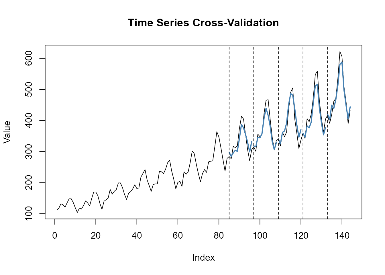
The tuning procedure uses rolling-origin evaluation with expanding
training windows. Here, n_ahead = 12 produces 12-step-ahead
forecasts, and n_split = 5 creates five rolling train/test
splits. For each split and each hyperparameter combination, the model is
fitted on the training window and evaluated on the subsequent test
window. The resulting object stores the validation errors, including
mean squared error (MSE) and mean absolute error (MAE), for each
candidate configuration and split. Runtime increases with the number of
grid combinations and validation splits, so coarse grids are recommended
as a starting point before moving to finer tuning ranges.
The S3 method summary() reports the best hyperparameter
set according to the default accuracy metric (MSE unless you specify
metric = "mae"), along with the corresponding performance.
plot() visualizes the actual data together with the point
forecasts from the selected “best” configuration. Forecasts are drawn as
separate line segments over each test window, and vertical dashed lines
indicate where each test window begins, making it easy to see how
performance varies across splits.
# Tune hyperparameters via time series cross-validation
xfit <- tune_esn(
  y = xdata,
  n_ahead = 12,
  n_split = 5,
  alpha = seq(0.1, 1.0, 0.1),
  rho   = c(1.0),
  tau   = c(0.4)
)

# Summarize and visualize optimal hyperparameter configuration
summary(xfit)
#> # A tibble: 5 × 11
#>   alpha   rho   tau split train_start train_end test_start test_end   mse   mae
#>   <dbl> <dbl> <dbl> <int>       <int>     <int>      <int>    <int> <dbl> <dbl>
#> 1     1     1   0.4     1           1        84         85       96  471.  19.5
#> 2     1     1   0.4     2           1        96         97      108  376.  14.2
#> 3     1     1   0.4     3           1       108        109      120  526.  19.0
#> 4     1     1   0.4     4           1       120        121      132  547.  20.2
#> 5     1     1   0.4     5           1       132        133      144  396.  17.0
#> # ℹ 1 more variable: id <int>
plot(xfit)