Prepare dataset
In this example, we will use the m4_monthly_subset. The
dataset is a monthly tsibble, which is filtered to include
only the time series "M21655" and "M2717". The
resulting object train_frame contains the training data and
is visualized below.
train_frame <- m4_monthly_subset %>%
  filter(series %in% c("M21655", "M2717"))

train_frame
#> # A tsibble: 494 x 4 [1M]
#> # Key:       series [2]
#>    series category       index value
#>    <chr>  <fct>          <mth> <dbl>
#>  1 M21655 Demographic 1995 Jan  4970
#>  2 M21655 Demographic 1995 Feb  5010
#>  3 M21655 Demographic 1995 Mrz  5060
#>  4 M21655 Demographic 1995 Apr  5010
#>  5 M21655 Demographic 1995 Mai  5610
#>  6 M21655 Demographic 1995 Jun  6040
#>  7 M21655 Demographic 1995 Jul  6450
#>  8 M21655 Demographic 1995 Aug  6370
#>  9 M21655 Demographic 1995 Sep  5190
#> 10 M21655 Demographic 1995 Okt  5250
#> # ℹ 484 more rows

p <- ggplot()

p <- p + geom_line(
  data = train_frame,
  aes(
    x = index,
    y = value),
  linewidth = 0.5
)

p <- p + facet_wrap(
  vars(series),
  ncol = 1,
  scales = "free")

p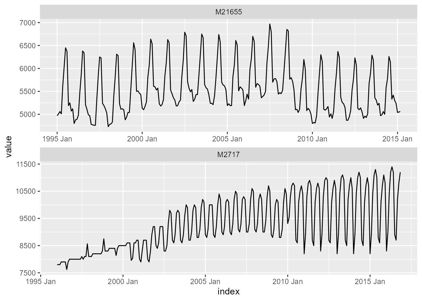
Train ESN model
The function ESN() is used in combination with
model() from the fabletools package to train
an Echo State Network for the variable value. The trained
models are stored as a mable (i.e., model table).
Additionally, an ARIMA() model is trained as a
benchmark.
mable_frame <- train_frame %>%
  model(
    "ESN" = ESN(value),
    "ARIMA" = ARIMA(value)
    )

mable_frame
#> # A mable: 2 x 3
#> # Key:     series [2]
#>   series                              ESN                     ARIMA
#>   <chr>                           <model>                   <model>
#> 1 M21655   <ESN({97, 1, 1}, {194, 25.8})> <ARIMA(1,0,0)(1,1,2)[12]>
#> 2 M2717  <ESN({100, 1, 1}, {200, 28.78})> <ARIMA(2,1,4)(0,1,0)[12]>
Forecast ESN model
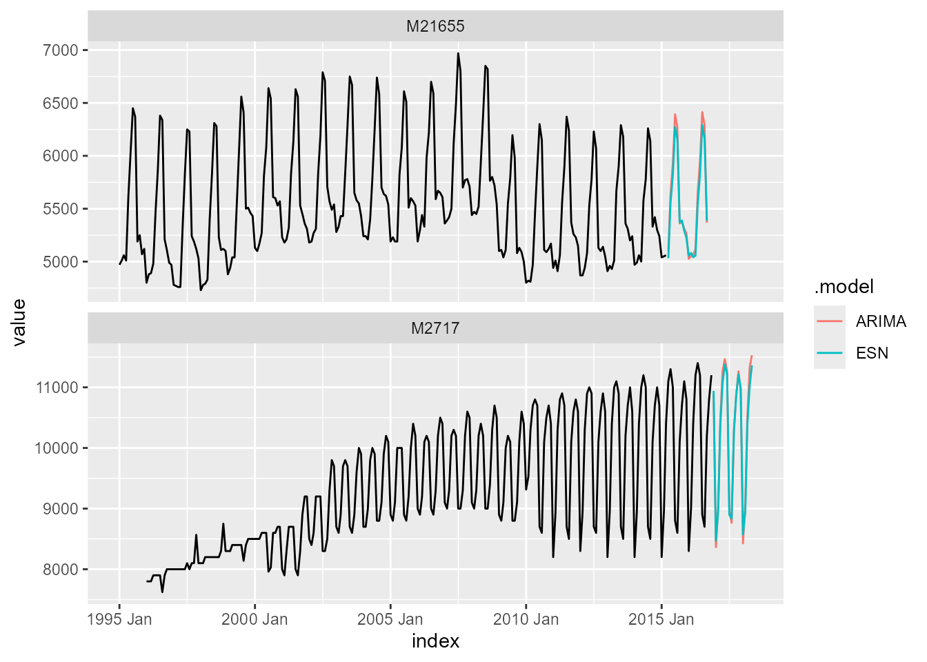
Forecasts are generated via the function forecast(),
where the forecast horizon is set to h = 18 (i.e.,
18-month-ahead forecasts). The forecasts are stored as a
fable (i.e., forecast table) and visualized along
the historical training data.
fable_frame <- mable_frame %>%
  forecast(h = 18)

fable_frame
#> # A fable: 72 x 5 [1M]
#> # Key:     series, .model [4]
#>    series .model    index
#>    <chr>  <chr>     <mth>
#>  1 M21655 ESN    2015 Apr
#>  2 M21655 ESN    2015 Mai
#>  3 M21655 ESN    2015 Jun
#>  4 M21655 ESN    2015 Jul
#>  5 M21655 ESN    2015 Aug
#>  6 M21655 ESN    2015 Sep
#>  7 M21655 ESN    2015 Okt
#>  8 M21655 ESN    2015 Nov
#>  9 M21655 ESN    2015 Dez
#> 10 M21655 ESN    2016 Jan
#> # ℹ 62 more rows
#> # ℹ 2 more variables: value <dist>, .mean <dbl>

fable_frame %>%
  autoplot(train_frame, level = NULL)
#> Warning: `autoplot.fbl_ts()` was deprecated in fabletools 0.6.0.
#> ℹ Please use `ggtime::autoplot.fbl_ts()` instead.
#> ℹ Graphics functions have been moved to the {ggtime} package. Please use
#>   `library(ggtime)` instead.
#> This warning is displayed once per session.
#> Call `lifecycle::last_lifecycle_warnings()` to see where this warning was
#> generated.