Time Series Cross Validation with M4 Monthly Data

The package tscv provides a collection of functions and tools for time series analysis and forecasting as well as time series cross-validation. This is mainly a set of wrapper and helper functions as well as some extensions for the packages tsibble, fable and fabletools that I find useful for research in the area of time series forecasting.

Disclaimer: The tscv package is highly experimental and it is very likely that there will be (substantial) changes in the near future.

Installation

You can install the development version from GitHub with:

# install.packages("devtools")
devtools::install_github("ahaeusser/tscv")

Example

# Load relevant packages
library(tscv)
library(tidyverse)
library(tsibble)
library(fable)
library(feasts)

Data preparation

The data set M4_monthly_data is a tibble with selected monthly time series from the M4 forecasting competition. It contains the following columns:

index: monthly time index
series: time series ID from the M4 forecasting competition
category: category from the M4 forecasting competition
value: measurement variable

In this vignette, we use two monthly time series, M10960 and M23100, to demonstrate time series cross-validation with a fixed window approach and an 18-month-ahead forecast horizon. You can use the function plot_line() to visualize the two time series. The function summarise_data() is used to explore the structure (start date, end date, number of observations and the number missing and zero values). The function summarise_stats() calculates descriptive statistics for each time series.


series_id = "series"
value_id = "value"
index_id = "index"

context <- list(
  series_id = series_id,
  value_id = value_id,
  index_id = index_id
)

# Prepare data set
main_frame <- M4_monthly_data |>
  filter(series %in% c("M10960", "M23100"))

main_frame
#> # A tibble: 492 × 4
#>       index series category value
#>       <mth> <chr>  <chr>    <dbl>
#>  1 1990 Jan M10960 Micro     2040
#>  2 1990 Feb M10960 Micro     1977
#>  3 1990 Mar M10960 Micro     1966
#>  4 1990 Apr M10960 Micro     1955
#>  5 1990 May M10960 Micro     1959
#>  6 1990 Jun M10960 Micro     1979
#>  7 1990 Jul M10960 Micro     2015
#>  8 1990 Aug M10960 Micro     2011
#>  9 1990 Sep M10960 Micro     2007
#> 10 1990 Oct M10960 Micro     2037
#> # ℹ 482 more rows

main_frame |>
  plot_line(
    x = index,
    y = value,
    color = series,
    facet_var = series,
    title = "M4 Monthly Time Series",
    subtitle = "Series M10960 and M23100",
    xlab = "Time",
    ylab = "Value",
    caption = "Data: M4 Competition"
    )
#> Warning: Using `size` aesthetic for lines was deprecated in ggplot2 3.4.0.
#> ℹ Please use `linewidth` instead.
#> ℹ The deprecated feature was likely used in the tscv package.
#>   Please report the issue at <https://github.com/ahaeusser/tscv/issues>.
#> This warning is displayed once per session.
#> Call `lifecycle::last_lifecycle_warnings()` to see where this warning was
#> generated.
#> Warning: The `size` argument of `element_line()` is deprecated as of ggplot2 3.4.0.
#> ℹ Please use the `linewidth` argument instead.
#> ℹ The deprecated feature was likely used in the tscv package.
#>   Please report the issue at <https://github.com/ahaeusser/tscv/issues>.
#> This warning is displayed once per session.
#> Call `lifecycle::last_lifecycle_warnings()` to see where this warning was
#> generated.
#> Warning: The `size` argument of `element_rect()` is deprecated as of ggplot2 3.4.0.
#> ℹ Please use the `linewidth` argument instead.
#> ℹ The deprecated feature was likely used in the tscv package.
#>   Please report the issue at <https://github.com/ahaeusser/tscv/issues>.
#> This warning is displayed once per session.
#> Call `lifecycle::last_lifecycle_warnings()` to see where this warning was
#> generated.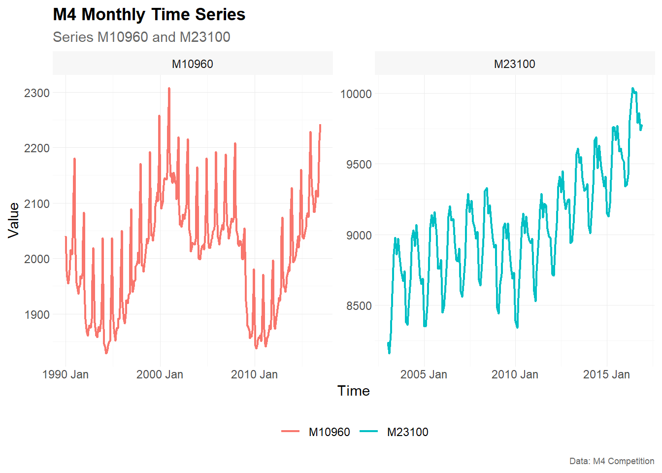

Plot raw M4 monthly data


summarise_data(
  .data = main_frame,
  context = context
)
#> # A tibble: 2 × 8
#>   series    start      end n_obs n_missing pct_missing n_zeros pct_zeros
#>   <chr>     <mth>    <mth> <int>     <int>       <dbl>   <int>     <dbl>
#> 1 M10960 1990 Jan 2016 Dec   324         0           0       0         0
#> 2 M23100 2003 Jan 2016 Dec   168         0           0       0         0

summarise_stats(
  .data = main_frame,
  context = context
)
#> # A tibble: 2 × 11
#>   series  mean median  mode    sd    p0   p25   p75  p100 skewness kurtosis
#>   <chr>  <dbl>  <dbl> <dbl> <dbl> <dbl> <dbl> <dbl> <dbl>    <dbl>    <dbl>
#> 1 M10960 2008.   2022 2035.  101.  1829 1924. 2072.  2308    0.129     2.36
#> 2 M23100 9059.   9050 9040.  394.  8160 8768. 9310  10040    0.222     2.74

Split data into training and testing

To prepare the data set for time series cross-validation (TSCV), you can use the function make_split(). This function splits the data into several slices for training and testing (i.e. partitioning into time slices) for time series cross-validation. You can choose between stretch and slide. The first is an expanding window approach, while the latter is a fixed window approach. Furthermore, we define the (initial) window size for training and testing via n_init and n_ahead, as well as the step size for increments via n_skip. Further options for splitting the data are available via type (see function reference for more details).

In this vignette, we use a fixed window approach with a 120-month training window and an 18-month testing window. The value n_skip = 17 creates non-overlapping 18-month test windows.


# Setup for time series cross validation
type = "first"
value = 120       # size for training window (= 10 years of monthly observations)
n_ahead = 18      # size for testing window (= forecast horizon, 18 months ahead)
n_skip = 17       # skip 17 observations to obtain non-overlapping test windows
n_lag = 0         # no lag
mode = "slide"    # fixed window approach
exceed = FALSE    # only pseudo out-of-sample forecast

split_frame <- make_split(
  main_frame = main_frame,
  context = context,
  type = type,
  value = value,
  n_ahead = n_ahead,
  n_skip = n_skip,
  n_lag = n_lag,
  mode = mode,
  exceed = exceed
)

split_frame
#> # A tibble: 13 × 4
#>    series split train       test      
#>    <chr>  <int> <list>      <list>    
#>  1 M10960     1 <int [120]> <int [18]>
#>  2 M10960     2 <int [120]> <int [18]>
#>  3 M10960     3 <int [120]> <int [18]>
#>  4 M10960     4 <int [120]> <int [18]>
#>  5 M10960     5 <int [120]> <int [18]>
#>  6 M10960     6 <int [120]> <int [18]>
#>  7 M10960     7 <int [120]> <int [18]>
#>  8 M10960     8 <int [120]> <int [18]>
#>  9 M10960     9 <int [120]> <int [18]>
#> 10 M10960    10 <int [120]> <int [18]>
#> 11 M10960    11 <int [120]> <int [18]>
#> 12 M23100     1 <int [120]> <int [18]>
#> 13 M23100     2 <int [120]> <int [18]>

Training and forecasting

The training and test splits are prepared within split_frame and we are ready for forecasting. The function slice_train() slices the data main_frame according to the splits within split_frame. As we are using forecasting methods from the packages fable and fabletools, we have to convert the data set main_frame from a tibble to a tsibble.

For the monthly M4 data, we use simple benchmark and automatic forecasting methods:

NAIVE: naive random walk model
SNAIVE: seasonal naive model with yearly seasonality
STL-NAIVE: STL-decomposition model and naive forecast. The series is decomposed via STL and the seasonally adjusted series is predicted via the naive approach. Afterwards, the seasonal component is added to the forecasts
ETS: exponential smoothing state space model
ARIMA: automatic ARIMA model
SMEDIAN: seasonal median model with yearly seasonality

The function SMEDIAN() is an extension to the fable package.


# Slice training data from main_frame according to split_frame
train_frame <- slice_train(
  main_frame = main_frame,
  split_frame = split_frame,
  context = context
  )

train_frame
#> # A tibble: 1,560 × 5
#>       index series category value split
#>       <mth> <chr>  <chr>    <dbl> <int>
#>  1 1990 Jan M10960 Micro     2040     1
#>  2 1990 Feb M10960 Micro     1977     1
#>  3 1990 Mar M10960 Micro     1966     1
#>  4 1990 Apr M10960 Micro     1955     1
#>  5 1990 May M10960 Micro     1959     1
#>  6 1990 Jun M10960 Micro     1979     1
#>  7 1990 Jul M10960 Micro     2015     1
#>  8 1990 Aug M10960 Micro     2011     1
#>  9 1990 Sep M10960 Micro     2007     1
#> 10 1990 Oct M10960 Micro     2037     1
#> # ℹ 1,550 more rows

# Convert tibble to tsibble
train_frame <- train_frame |>
  as_tsibble(
    index = index,
    key = c(series, split)
    )

train_frame
#> # A tsibble: 1,560 x 5 [1M]
#> # Key:       series, split [13]
#>       index series category value split
#>       <mth> <chr>  <chr>    <dbl> <int>
#>  1 1990 Jan M10960 Micro     2040     1
#>  2 1990 Feb M10960 Micro     1977     1
#>  3 1990 Mar M10960 Micro     1966     1
#>  4 1990 Apr M10960 Micro     1955     1
#>  5 1990 May M10960 Micro     1959     1
#>  6 1990 Jun M10960 Micro     1979     1
#>  7 1990 Jul M10960 Micro     2015     1
#>  8 1990 Aug M10960 Micro     2011     1
#>  9 1990 Sep M10960 Micro     2007     1
#> 10 1990 Oct M10960 Micro     2037     1
#> # ℹ 1,550 more rows

# Model training via fabletools::model()
model_frame <- train_frame |>
  model(
    "NAIVE" = NAIVE(value),
    "SNAIVE" = SNAIVE(value ~ lag("year")),
    "STL-NAIVE" = decomposition_model(STL(value), NAIVE(season_adjust)),
    "ETS" = ETS(value),
    "ARIMA" = ARIMA(value),
    "SMEDIAN" = SMEDIAN(value ~ lag("year"))
    )

model_frame
#> # A mable: 13 x 8
#> # Key:     series, split [13]
#>    series split   NAIVE   SNAIVE               `STL-NAIVE`           ETS
#>    <chr>  <int> <model>  <model>                   <model>       <model>
#>  1 M10960     1 <NAIVE> <SNAIVE> <STL decomposition model>  <ETS(M,A,A)>
#>  2 M10960     2 <NAIVE> <SNAIVE> <STL decomposition model>  <ETS(A,A,A)>
#>  3 M10960     3 <NAIVE> <SNAIVE> <STL decomposition model>  <ETS(M,N,A)>
#>  4 M10960     4 <NAIVE> <SNAIVE> <STL decomposition model>  <ETS(M,A,A)>
#>  5 M10960     5 <NAIVE> <SNAIVE> <STL decomposition model> <ETS(M,Ad,A)>
#>  6 M10960     6 <NAIVE> <SNAIVE> <STL decomposition model> <ETS(M,Ad,A)>
#>  7 M10960     7 <NAIVE> <SNAIVE> <STL decomposition model> <ETS(M,Ad,M)>
#>  8 M10960     8 <NAIVE> <SNAIVE> <STL decomposition model> <ETS(M,Ad,M)>
#>  9 M10960     9 <NAIVE> <SNAIVE> <STL decomposition model> <ETS(M,Ad,M)>
#> 10 M10960    10 <NAIVE> <SNAIVE> <STL decomposition model>  <ETS(M,N,A)>
#> 11 M10960    11 <NAIVE> <SNAIVE> <STL decomposition model>  <ETS(M,N,A)>
#> 12 M23100     1 <NAIVE> <SNAIVE> <STL decomposition model> <ETS(M,Ad,A)>
#> 13 M23100     2 <NAIVE> <SNAIVE> <STL decomposition model>  <ETS(A,A,A)>
#> # ℹ 2 more variables: ARIMA <model>, SMEDIAN <model>

# Forecasting via fabletools::forecast()
fable_frame <- model_frame |>
  forecast(h = n_ahead)

fable_frame
#> # A fable: 1,404 x 6 [1M]
#> # Key:     series, split, .model [78]
#>    series split .model    index
#>    <chr>  <int> <chr>     <mth>
#>  1 M10960     1 NAIVE  2000 Jan
#>  2 M10960     1 NAIVE  2000 Feb
#>  3 M10960     1 NAIVE  2000 Mar
#>  4 M10960     1 NAIVE  2000 Apr
#>  5 M10960     1 NAIVE  2000 May
#>  6 M10960     1 NAIVE  2000 Jun
#>  7 M10960     1 NAIVE  2000 Jul
#>  8 M10960     1 NAIVE  2000 Aug
#>  9 M10960     1 NAIVE  2000 Sep
#> 10 M10960     1 NAIVE  2000 Oct
#> # ℹ 1,394 more rows
#> # ℹ 2 more variables: value <dist>, .mean <dbl>

# Convert fable_frame (fable) to future_frame (tibble)
future_frame <- make_future(
  fable = fable_frame,
  context = context
  )

future_frame
#> # A tibble: 1,404 × 6
#>       index series model split horizon point
#>       <mth> <chr>  <chr> <int>   <int> <dbl>
#>  1 2000 Jan M10960 NAIVE     1       1  2258
#>  2 2000 Feb M10960 NAIVE     1       2  2258
#>  3 2000 Mar M10960 NAIVE     1       3  2258
#>  4 2000 Apr M10960 NAIVE     1       4  2258
#>  5 2000 May M10960 NAIVE     1       5  2258
#>  6 2000 Jun M10960 NAIVE     1       6  2258
#>  7 2000 Jul M10960 NAIVE     1       7  2258
#>  8 2000 Aug M10960 NAIVE     1       8  2258
#>  9 2000 Sep M10960 NAIVE     1       9  2258
#> 10 2000 Oct M10960 NAIVE     1      10  2258
#> # ℹ 1,394 more rows

Evaluation of forecast accuracy

To evaluate the forecast accuracy, the function make_accuracy() is used. You can define whether to evaluate the accuracy by horizon or by split. Several accuracy metrics are available:

ME: mean error
MAE: mean absolute error
MSE: mean squared error
RMSE: root mean squared error
MAPE: mean absolute percentage error
sMAPE: scaled mean absolute percentage error
MPE: mean percentage error
rMAE: relative mean absolute error (relative to some user-defined benchmark method)

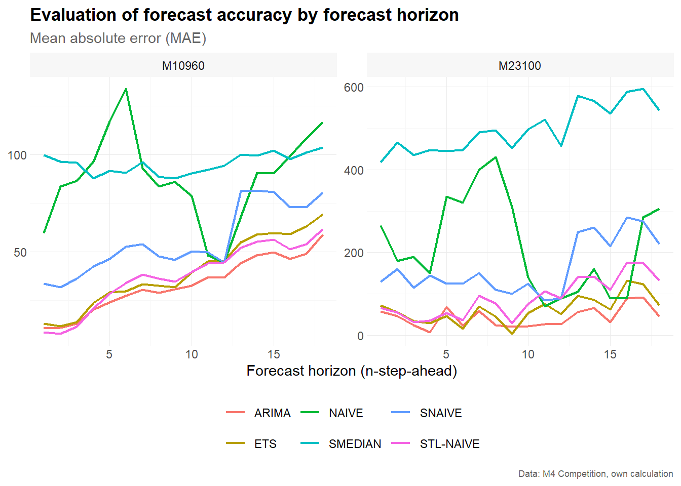
Forecast accuracy by forecast horizon


# Estimate accuracy metrics by forecast horizon
accuracy_horizon <- make_accuracy(
  future_frame = future_frame,
  main_frame = main_frame,
  context = context,
  dimension = "horizon"
)

accuracy_horizon
#> # A tibble: 1,512 × 6
#>    series model dimension     n metric value
#>    <chr>  <chr> <chr>     <int> <chr>  <dbl>
#>  1 M10960 ARIMA horizon       1 MAE     10.4
#>  2 M10960 ARIMA horizon       2 MAE     10.8
#>  3 M10960 ARIMA horizon       3 MAE     12.8
#>  4 M10960 ARIMA horizon       4 MAE     20.2
#>  5 M10960 ARIMA horizon       5 MAE     23.9
#>  6 M10960 ARIMA horizon       6 MAE     27.3
#>  7 M10960 ARIMA horizon       7 MAE     30.3
#>  8 M10960 ARIMA horizon       8 MAE     28.9
#>  9 M10960 ARIMA horizon       9 MAE     30.5
#> 10 M10960 ARIMA horizon      10 MAE     32.6
#> # ℹ 1,502 more rows

# Visualize results
accuracy_horizon |>
  filter(metric == "MAE") |>
  plot_line(
    x = n,
    y = value,
    facet_var = series,
    facet_nrow = 1,
    color = model,
    title = "Evaluation of forecast accuracy by forecast horizon",
    subtitle = "Mean absolute error (MAE)",
    xlab = "Forecast horizon (n-step-ahead)",
    caption = "Data: M4 Competition, own calculation"
    )

Plot accuracy by horizon

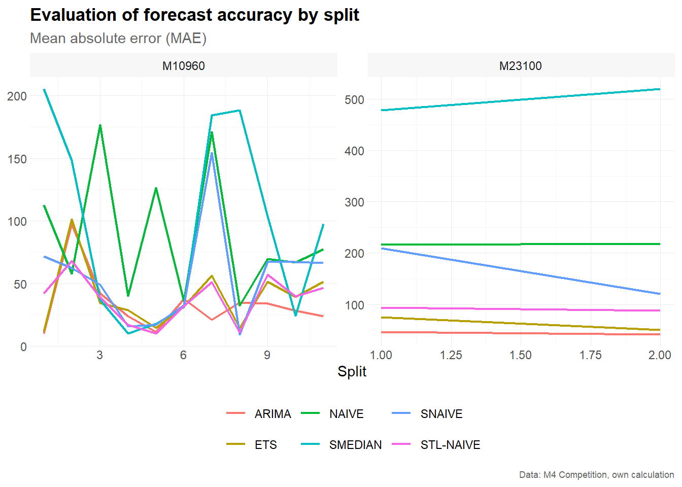
Forecast accuracy by split


# Estimate accuracy metrics by split
accuracy_split <- make_accuracy(
  future_frame = future_frame,
  main_frame = main_frame,
  context = context,
  dimension = "split"
)

accuracy_split
#> # A tibble: 546 × 6
#>    series model dimension     n metric value
#>    <chr>  <chr> <chr>     <int> <chr>  <dbl>
#>  1 M10960 ARIMA split         1 MAE     9.97
#>  2 M10960 ARIMA split         2 MAE    97.4 
#>  3 M10960 ARIMA split         3 MAE    42.3 
#>  4 M10960 ARIMA split         4 MAE    24.0 
#>  5 M10960 ARIMA split         5 MAE    11.4 
#>  6 M10960 ARIMA split         6 MAE    37.8 
#>  7 M10960 ARIMA split         7 MAE    21.0 
#>  8 M10960 ARIMA split         8 MAE    34.9 
#>  9 M10960 ARIMA split         9 MAE    34.0 
#> 10 M10960 ARIMA split        10 MAE    28.3 
#> # ℹ 536 more rows

# Visualize results
accuracy_split |>
  filter(metric == "MAE") |>
  plot_line(
    x = n,
    y = value,
    facet_var = series,
    facet_nrow = 1,
    color = model,
    title = "Evaluation of forecast accuracy by split",
    subtitle = "Mean absolute error (MAE)",
    xlab = "Split",
    caption = "Data: M4 Competition, own calculation"
    )

Plot accuracy by split

Alexander Häußer

April 2026