Expanding window approach

The package tscv provides helper functions for time series analysis, forecasting and time series cross-validation. It is mainly designed to work with the tidy forecasting ecosystem, especially the packages tsibble, fable, fabletools and feasts.

In this vignette, we demonstrate an expanding window approach for time series cross-validation using monthly time series from the M4 forecasting competition.

Installation

You can install the development version from GitHub with:

# install.packages("devtools")
devtools::install_github("ahaeusser/tscv")

Example

# Load relevant packages
library(tscv)
library(tidyverse)
library(tsibble)
library(fable)
library(feasts)

Data preparation

The data set M4_monthly_data is a tibble with selected monthly time series from the M4 forecasting competition. It contains the following columns:

index: monthly time index
series: time series ID from the M4 forecasting competition
category: category from the M4 forecasting competition
value: measurement variable

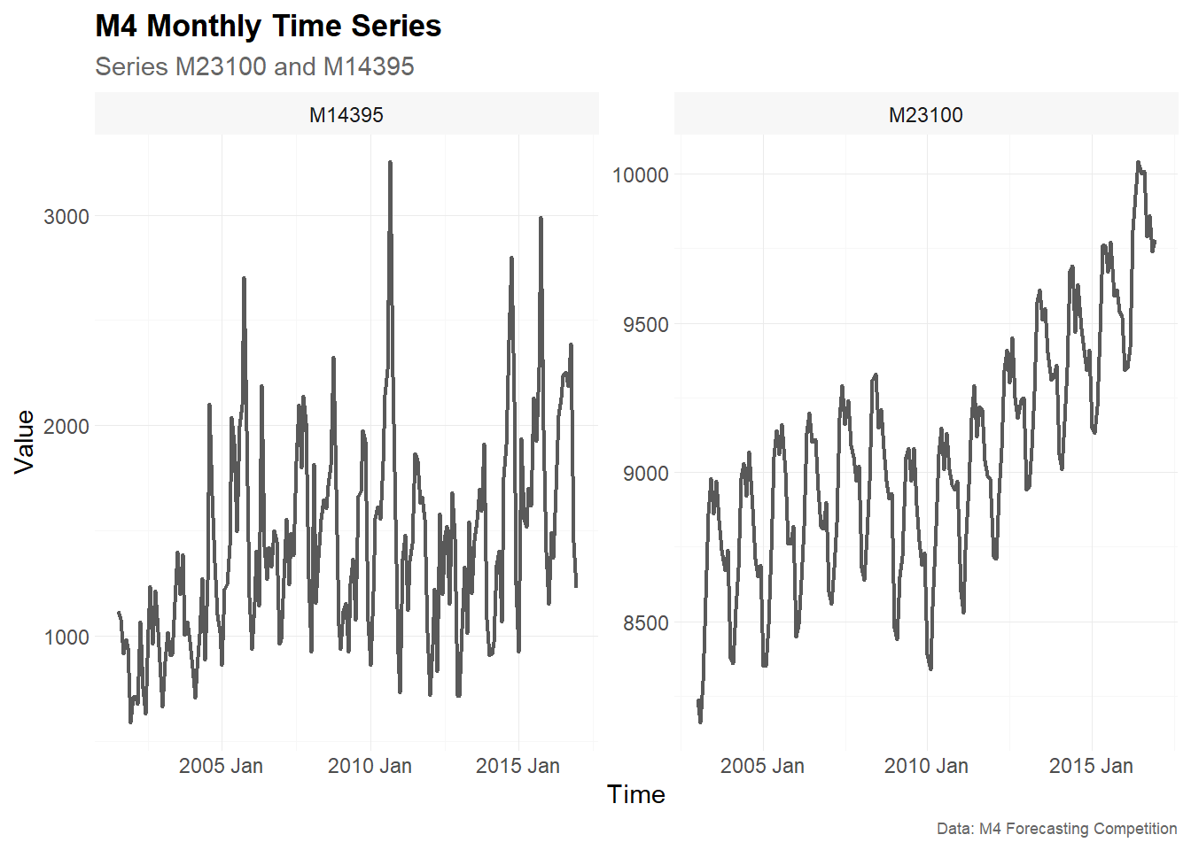
In this vignette, we use two monthly time series, M23100 and M14395, to demonstrate time series cross-validation with an expanding window approach and an 18-month-ahead forecast horizon.

The function plot_line() is used to visualize the time series. The function summarise_data() explores the structure of the data, including the start date, end date, number of observations, number of missing values and number of zero values. The function summarise_stats() calculates descriptive statistics for each time series.

series_id = "series"
value_id = "value"
index_id = "index"

context <- list(
  series_id = series_id,
  value_id = value_id,
  index_id = index_id
)

# Prepare data set
main_frame <- M4_monthly_data |>
  filter(series %in% c("M23100", "M14395"))

main_frame
#> # A tibble: 354 × 4
#>       index series category value
#>       <mth> <chr>  <chr>    <dbl>
#>  1 2001 Jul M14395 Micro    1116.
#>  2 2001 Aug M14395 Micro    1079.
#>  3 2001 Sep M14395 Micro     917.
#>  4 2001 Oct M14395 Micro     982.
#>  5 2001 Nov M14395 Micro     946.
#>  6 2001 Dec M14395 Micro     586.
#>  7 2002 Jan M14395 Micro     710.
#>  8 2002 Feb M14395 Micro     714.
#>  9 2002 Mar M14395 Micro     675 
#> 10 2002 Apr M14395 Micro    1068.
#> # ℹ 344 more rows

main_frame |>
  plot_line(
    x = index,
    y = value,
    facet_var = series,
    title = "M4 Monthly Time Series",
    subtitle = "Series M23100 and M14395",
    xlab = "Time",
    ylab = "Value",
    caption = "Data: M4 Forecasting Competition"
  )

Plot raw M4 monthly data


summarise_data(
  .data = main_frame,
  context = context
)
#> # A tibble: 2 × 8
#>   series    start      end n_obs n_missing pct_missing n_zeros pct_zeros
#>   <chr>     <mth>    <mth> <int>     <int>       <dbl>   <int>     <dbl>
#> 1 M14395 2001 Jul 2016 Dec   186         0           0       0         0
#> 2 M23100 2003 Jan 2016 Dec   168         0           0       0         0

summarise_stats(
  .data = main_frame,
  context = context
)
#> # A tibble: 2 × 11
#>   series  mean median  mode    sd    p0   p25   p75  p100 skewness kurtosis
#>   <chr>  <dbl>  <dbl> <dbl> <dbl> <dbl> <dbl> <dbl> <dbl>    <dbl>    <dbl>
#> 1 M14395 1422.  1369. 1113.  490.  586. 1031. 1697.  3253    0.786     3.62
#> 2 M23100 9059.  9050  9040.  394. 8160  8768. 9310  10040    0.222     2.74

Split data into training and testing

To prepare the data for time series cross-validation, we use the function make_split(). This function partitions the data into several training and testing slices.

The argument mode controls the type of rolling-origin resampling:

mode = "stretch" creates an expanding window.
mode = "slide" creates a fixed window.

In an expanding window approach, the training sample grows over time. The first split starts with an initial training window of fixed length. In later splits, additional observations are added to the training sample, while the forecast horizon remains unchanged.

In this vignette, we use:

value = 120: the first training window contains 120 monthly observations, corresponding to 10 years of data
n_ahead = 18: each test set contains 18 observations, corresponding to an 18-month-ahead forecast horizon
n_skip = 17: after each split, the rolling origin is advanced by 18 months, which creates non-overlapping test windows
mode = "stretch": the training window expands over time

# Setup for time series cross validation
type = "first"
value = 120       # initial training window (= 10 years of monthly observations)
n_ahead = 18      # testing window (= forecast horizon, 18 months ahead)
n_skip = 17       # skip 17 observations to obtain non-overlapping test windows
n_lag = 0         # no lag
mode = "stretch"  # expanding window approach
exceed = FALSE    # only pseudo out-of-sample forecast

split_frame <- make_split(
  main_frame = main_frame,
  context = context,
  type = type,
  value = value,
  n_ahead = n_ahead,
  n_skip = n_skip,
  n_lag = n_lag,
  mode = mode,
  exceed = exceed
)

split_frame
#> # A tibble: 5 × 4
#>   series split train       test      
#>   <chr>  <int> <list>      <list>    
#> 1 M14395     1 <int [120]> <int [18]>
#> 2 M14395     2 <int [138]> <int [18]>
#> 3 M14395     3 <int [156]> <int [18]>
#> 4 M23100     1 <int [120]> <int [18]>
#> 5 M23100     2 <int [138]> <int [18]>

The resulting object split_frame contains one row per time series and split. The columns train and test are list-columns containing the row positions used for the training and test samples.

The output above shows that the first split uses 120 observations for training and 18 observations for testing. In the second split, the training window has expanded to 138 observations, while the test window remains fixed at 18 observations. The third split for series M14395 uses 156 observations for training.

The number of splits can differ across time series because the selected M4 series do not necessarily have the same number of observations. In the example above, M14395 allows three valid 18-month test windows, while M23100 allows two.

Training and forecasting

The training and test samples are defined in split_frame. We now use slice_train() and slice_test() to extract the corresponding observations from main_frame.

Since the forecasting models are estimated with functions from fable and fabletools, the training data is converted from a tibble to a tsibble.

For the monthly M4 data, we estimate three forecasting models:

SNAIVE: seasonal naive model with yearly seasonality
ETS: exponential smoothing state space model
ARIMA: automatic ARIMA model

These models are estimated separately for each time series and each split.

# Slice training data from main_frame according to split_frame
train_frame <- slice_train(
  main_frame = main_frame,
  split_frame = split_frame,
  context = context
)

train_frame
#> # A tibble: 672 × 5
#>       index series category value split
#>       <mth> <chr>  <chr>    <dbl> <int>
#>  1 2001 Jul M14395 Micro    1116.     1
#>  2 2001 Aug M14395 Micro    1079.     1
#>  3 2001 Sep M14395 Micro     917.     1
#>  4 2001 Oct M14395 Micro     982.     1
#>  5 2001 Nov M14395 Micro     946.     1
#>  6 2001 Dec M14395 Micro     586.     1
#>  7 2002 Jan M14395 Micro     710.     1
#>  8 2002 Feb M14395 Micro     714.     1
#>  9 2002 Mar M14395 Micro     675      1
#> 10 2002 Apr M14395 Micro    1068.     1
#> # ℹ 662 more rows

# Slice test data from main_frame according to split_frame
test_frame <- slice_test(
  main_frame = main_frame,
  split_frame = split_frame,
  context = context
)

test_frame
#> # A tibble: 90 × 5
#>       index series category value split
#>       <mth> <chr>  <chr>    <dbl> <int>
#>  1 2011 Jul M14395 Micro    1866.     1
#>  2 2011 Aug M14395 Micro    1833.     1
#>  3 2011 Sep M14395 Micro    1630.     1
#>  4 2011 Oct M14395 Micro    1659.     1
#>  5 2011 Nov M14395 Micro    1554.     1
#>  6 2011 Dec M14395 Micro    1018.     1
#>  7 2012 Jan M14395 Micro     717.     1
#>  8 2012 Feb M14395 Micro     958.     1
#>  9 2012 Mar M14395 Micro    1221.     1
#> 10 2012 Apr M14395 Micro     832.     1
#> # ℹ 80 more rows

# Convert tibble to tsibble
train_frame <- train_frame |>
  as_tsibble(
    index = index,
    key = c(series, split)
  )

train_frame
#> # A tsibble: 672 x 5 [1M]
#> # Key:       series, split [5]
#>       index series category value split
#>       <mth> <chr>  <chr>    <dbl> <int>
#>  1 2001 Jul M14395 Micro    1116.     1
#>  2 2001 Aug M14395 Micro    1079.     1
#>  3 2001 Sep M14395 Micro     917.     1
#>  4 2001 Oct M14395 Micro     982.     1
#>  5 2001 Nov M14395 Micro     946.     1
#>  6 2001 Dec M14395 Micro     586.     1
#>  7 2002 Jan M14395 Micro     710.     1
#>  8 2002 Feb M14395 Micro     714.     1
#>  9 2002 Mar M14395 Micro     675      1
#> 10 2002 Apr M14395 Micro    1068.     1
#> # ℹ 662 more rows

# Model training via fabletools::model()
model_frame <- train_frame |>
  model(
    "SNAIVE" = SNAIVE(value ~ lag("year")),
    "ETS" = ETS(value),
    "ARIMA" = ARIMA(value)
  )

model_frame
#> # A mable: 5 x 5
#> # Key:     series, split [5]
#>   series split   SNAIVE           ETS                              ARIMA
#>   <chr>  <int>  <model>       <model>                            <model>
#> 1 M14395     1 <SNAIVE>  <ETS(M,N,M)> <ARIMA(1,0,0)(0,1,1)[12] w/ drift>
#> 2 M14395     2 <SNAIVE>  <ETS(M,N,M)>          <ARIMA(1,0,1)(2,1,1)[12]>
#> 3 M14395     3 <SNAIVE>  <ETS(M,N,M)>          <ARIMA(0,0,2)(0,1,1)[12]>
#> 4 M23100     1 <SNAIVE> <ETS(M,Ad,A)> <ARIMA(1,0,0)(2,1,0)[12] w/ drift>
#> 5 M23100     2 <SNAIVE> <ETS(A,Ad,A)> <ARIMA(1,0,1)(2,1,0)[12] w/ drift>

# Forecasting via fabletools::forecast()
fable_frame <- model_frame |>
  forecast(h = n_ahead)

fable_frame
#> # A fable: 270 x 6 [1M]
#> # Key:     series, split, .model [15]
#>    series split .model    index
#>    <chr>  <int> <chr>     <mth>
#>  1 M14395     1 SNAIVE 2011 Jul
#>  2 M14395     1 SNAIVE 2011 Aug
#>  3 M14395     1 SNAIVE 2011 Sep
#>  4 M14395     1 SNAIVE 2011 Oct
#>  5 M14395     1 SNAIVE 2011 Nov
#>  6 M14395     1 SNAIVE 2011 Dec
#>  7 M14395     1 SNAIVE 2012 Jan
#>  8 M14395     1 SNAIVE 2012 Feb
#>  9 M14395     1 SNAIVE 2012 Mar
#> 10 M14395     1 SNAIVE 2012 Apr
#> # ℹ 260 more rows
#> # ℹ 2 more variables: value <dist>, .mean <dbl>

# Convert fable_frame (fable) to future_frame (tibble)
future_frame <- make_future(
  fable = fable_frame,
  context = context
)

future_frame
#> # A tibble: 270 × 6
#>       index series model  split horizon point
#>       <mth> <chr>  <chr>  <int>   <int> <dbl>
#>  1 2011 Jul M14395 SNAIVE     1       1 2145.
#>  2 2011 Aug M14395 SNAIVE     1       2 2264.
#>  3 2011 Sep M14395 SNAIVE     1       3 3253 
#>  4 2011 Oct M14395 SNAIVE     1       4 2232.
#>  5 2011 Nov M14395 SNAIVE     1       5 1556.
#>  6 2011 Dec M14395 SNAIVE     1       6  915.
#>  7 2012 Jan M14395 SNAIVE     1       7  732.
#>  8 2012 Feb M14395 SNAIVE     1       8 1367 
#>  9 2012 Mar M14395 SNAIVE     1       9 1478.
#> 10 2012 Apr M14395 SNAIVE     1      10 1122.
#> # ℹ 260 more rows

The object model_frame is a mable, that is, a model table. Each row corresponds to one combination of series and split, while each model is stored in a separate column.

The model specification may change across splits because the models are re-estimated for each training sample. This is especially visible for the automatic ETS() and ARIMA() models. For example, the selected ARIMA specification for M14395 differs between split 1, split 2 and split 3. This is expected, since each split uses a different training sample. The seasonal period [12] in the ARIMA output indicates yearly seasonality in monthly data.

Visualize rolling forecasts

To visualize the rolling forecasts, we combine the observed values and the forecasts into one data set.

The training and test observations are labelled as ACTUAL, while the forecasts keep their model names. The observed values are assigned horizon = 0, whereas the forecast values have horizons from 1 to 18.

# Combine actual values from train and test data
actual_frame <- bind_rows(
  train_frame,
  test_frame
)

# Combine actual values and forecasts
plot_frame <- bind_rows(
  actual_frame |>
    as_tibble() |>
    transmute(
      index,
      series,
      model = "ACTUAL",
      split,
      horizon = 0L,
      point = value
    ),
  future_frame
)

plot_frame
#> # A tibble: 1,032 × 6
#>       index series model  split horizon point
#>       <mth> <chr>  <chr>  <int>   <int> <dbl>
#>  1 2001 Jul M14395 ACTUAL     1       0 1116.
#>  2 2001 Aug M14395 ACTUAL     1       0 1079.
#>  3 2001 Sep M14395 ACTUAL     1       0  917.
#>  4 2001 Oct M14395 ACTUAL     1       0  982.
#>  5 2001 Nov M14395 ACTUAL     1       0  946.
#>  6 2001 Dec M14395 ACTUAL     1       0  586.
#>  7 2002 Jan M14395 ACTUAL     1       0  710.
#>  8 2002 Feb M14395 ACTUAL     1       0  714.
#>  9 2002 Mar M14395 ACTUAL     1       0  675 
#> 10 2002 Apr M14395 ACTUAL     1       0 1068.
#> # ℹ 1,022 more rows

The object plot_frame is useful for plotting actual observations and forecasts together. Since the data contains several rolling-origin splits, we facet the plots by split.

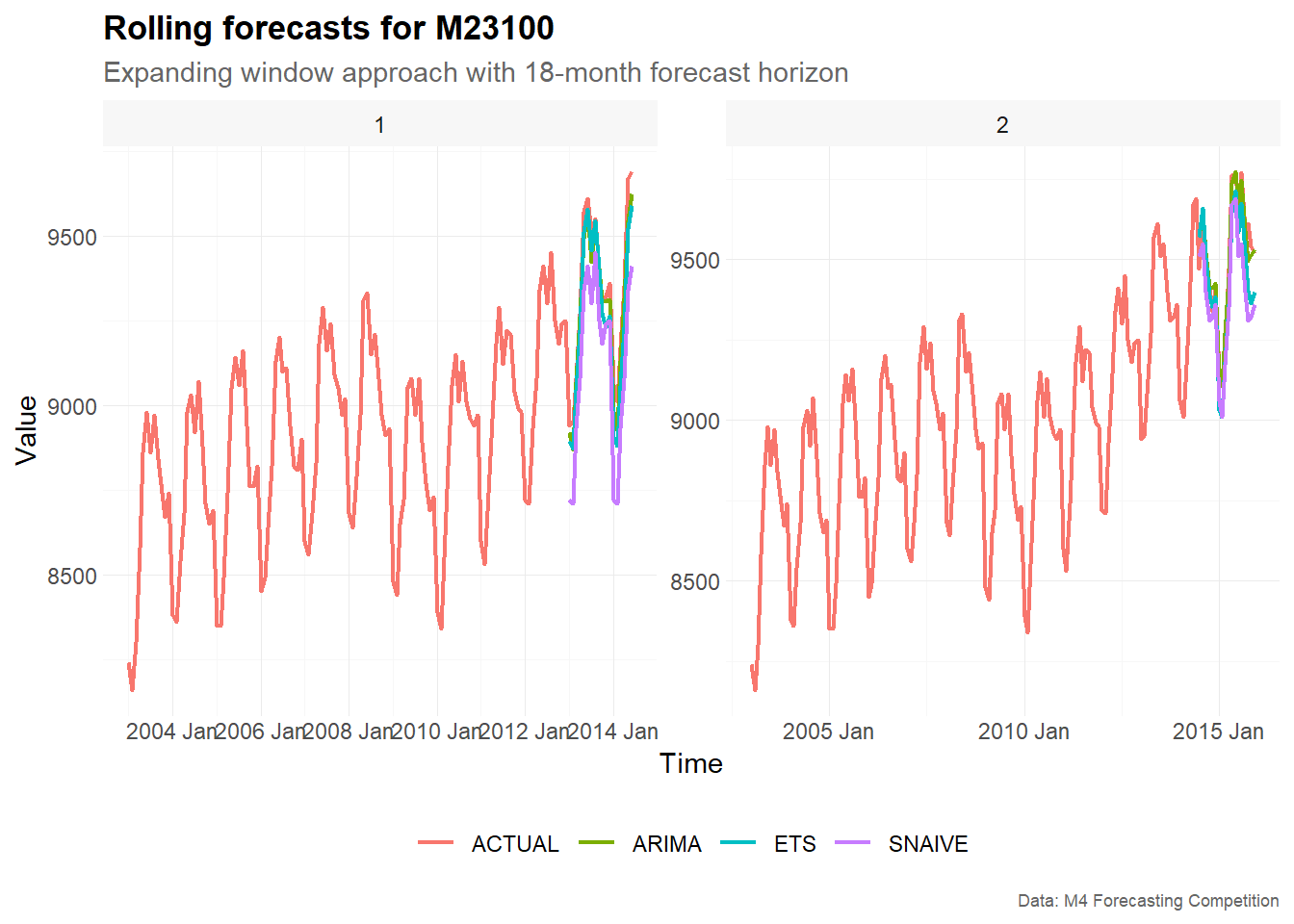
plot_frame |>
  filter(series == "M23100") |>
  plot_line(
    x = index,
    y = point,
    color = model,
    facet_var = split,
    title = "Rolling forecasts for M23100",
    subtitle = "Expanding window approach with 18-month forecast horizon",
    xlab = "Time",
    ylab = "Value",
    caption = "Data: M4 Forecasting Competition"
  )

Rolling forecasts for M23100

plot_frame |>
  filter(series == "M14395") |>
  plot_line(
    x = index,
    y = point,
    color = model,
    facet_var = split,
    title = "Rolling forecasts for M14395",
    subtitle = "Expanding window approach with 18-month forecast horizon",
    xlab = "Time",
    ylab = "Value",
    caption = "Data: M4 Forecasting Competition"
  )

Rolling forecasts for M14395

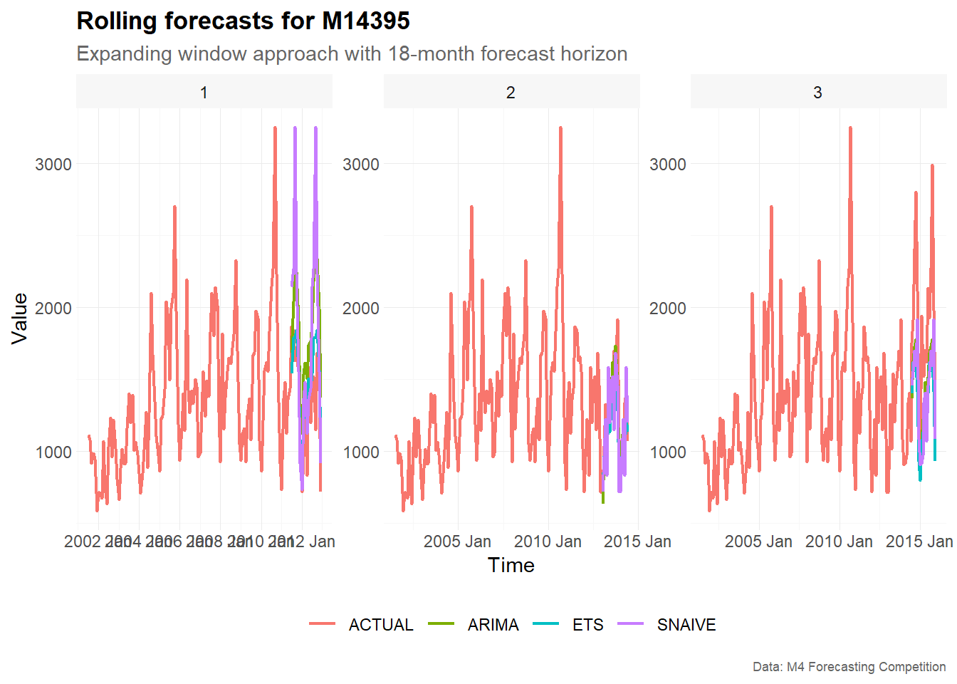
The plots show how the forecasts evolve across different rolling-origin splits. In each facet, the training window ends at a different point in time. The models are then estimated using only the available training data for that split and produce forecasts for the following 18 months.

Because we use an expanding window approach, later splits are based on larger training samples. This can lead to changes in the estimated model structure and in the resulting forecasts.

Forecast accuracy

The rolling forecasts can be evaluated against the test observations using make_accuracy(). Accuracy can be summarized either by forecast horizon or by split.

In this vignette, we focus on the symmetric mean absolute percentage error (sMAPE). The sMAPE is scale-independent and is therefore useful for comparing forecast accuracy across different time series.

Forecast accuracy by forecast horizon

Accuracy by forecast horizon shows how forecast errors change as the forecast horizon increases from 1 to 18 months ahead.

accuracy_horizon <- make_accuracy(
  future_frame = future_frame,
  main_frame = main_frame,
  context = context,
  dimension = "horizon"
)

accuracy_horizon |>
  filter(metric == "sMAPE")
#> # A tibble: 108 × 6
#>    series model dimension     n metric value
#>    <chr>  <chr> <chr>     <int> <chr>  <dbl>
#>  1 M14395 ARIMA horizon       1 sMAPE   15.7
#>  2 M14395 ARIMA horizon       2 sMAPE   11.2
#>  3 M14395 ARIMA horizon       3 sMAPE   28.8
#>  4 M14395 ARIMA horizon       4 sMAPE   26.2
#>  5 M14395 ARIMA horizon       5 sMAPE   18.9
#>  6 M14395 ARIMA horizon       6 sMAPE   17.1
#>  7 M14395 ARIMA horizon       7 sMAPE   19.7
#>  8 M14395 ARIMA horizon       8 sMAPE   35.8
#>  9 M14395 ARIMA horizon       9 sMAPE   19.2
#> 10 M14395 ARIMA horizon      10 sMAPE   30.9
#> # ℹ 98 more rows

Forecast accuracy by split

Accuracy by split shows how forecast errors vary across rolling-origin splits.

accuracy_split <- make_accuracy(
  future_frame = future_frame,
  main_frame = main_frame,
  context = context,
  dimension = "split"
)

accuracy_split |>
  filter(metric == "sMAPE")
#> # A tibble: 15 × 6
#>    series model  dimension     n metric  value
#>    <chr>  <chr>  <chr>     <int> <chr>   <dbl>
#>  1 M14395 ARIMA  split         1 sMAPE  33.8  
#>  2 M14395 ARIMA  split         2 sMAPE  12.8  
#>  3 M14395 ARIMA  split         3 sMAPE  27.9  
#>  4 M14395 ETS    split         1 sMAPE  15.8  
#>  5 M14395 ETS    split         2 sMAPE  13.9  
#>  6 M14395 ETS    split         3 sMAPE  34.6  
#>  7 M14395 SNAIVE split         1 sMAPE  27.3  
#>  8 M14395 SNAIVE split         2 sMAPE  15.2  
#>  9 M14395 SNAIVE split         3 sMAPE  29.0  
#> 10 M23100 ARIMA  split         1 sMAPE   0.501
#> 11 M23100 ARIMA  split         2 sMAPE   0.348
#> 12 M23100 ETS    split         1 sMAPE   0.816
#> 13 M23100 ETS    split         2 sMAPE   0.890
#> 14 M23100 SNAIVE split         1 sMAPE   2.28 
#> 15 M23100 SNAIVE split         2 sMAPE   1.27

The two accuracy views answer different questions. Accuracy by horizon is useful for understanding whether forecast performance changes with the forecast horizon. Accuracy by split is useful for identifying whether some forecast origins are more difficult than others.

Summary

This vignette demonstrated how to use tscv for time series cross-validation with an expanding window approach. The workflow consists of five main steps:

Prepare the data and define the column context.
Create rolling-origin splits using make_split().
Extract training and test samples using slice_train() and slice_test().
Estimate forecasting models and create forecasts.
Visualize and evaluate the rolling forecasts.

The expanding window approach is useful when the training sample should grow over time, which is often the case in real-world forecasting applications where all available historical information is used for model estimation.

Alexander Häußer

Mai 2026