Fixed window approach

The package tscv provides helper functions for time series analysis, forecasting and time series cross-validation. It is mainly designed to work with the tidy forecasting ecosystem, especially the packages tsibble, fable, fabletools and feasts.

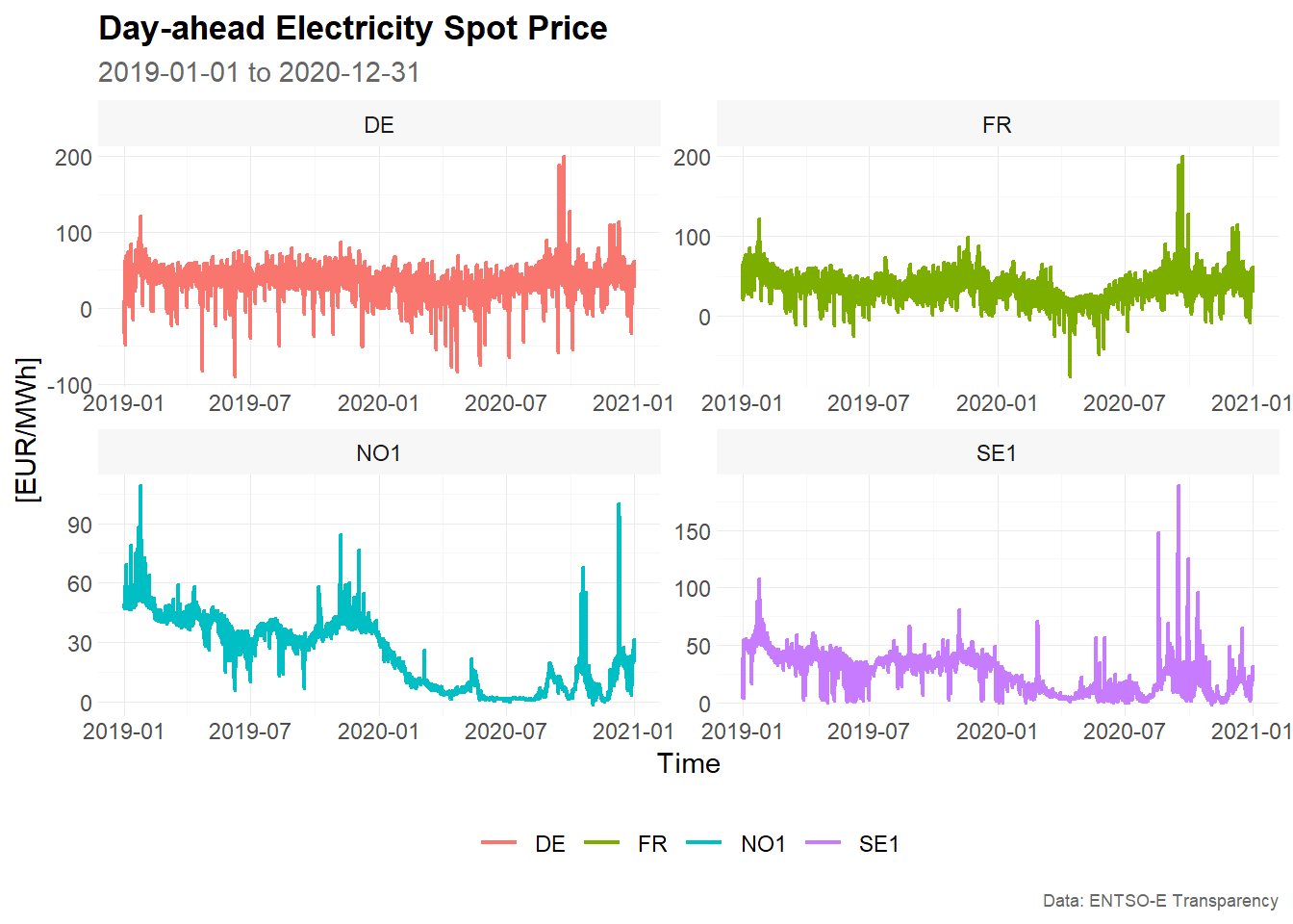
In this vignette, we demonstrate a fixed window approach for time series cross-validation using hourly day-ahead electricity spot prices.

Installation

You can install the development version from GitHub with:

# install.packages("devtools")
devtools::install_github("ahaeusser/tscv")

Example

# Load relevant packages
library(tscv)
library(tidyverse)
library(tsibble)
library(fable)
library(feasts)

Data preparation

The data set elec_price is a tibble with day-ahead electricity spot prices in [EUR/MWh] from the ENTSO-E Transparency Platform. The data set contains hourly time series data from 2019-01-01 to 2020-12-31 for eight European bidding zones:

DE: Germany, including Luxembourg
DK: Denmark
ES: Spain
FI: Finland
FR: France
NL: Netherlands
NO1: Norway 1, Oslo
SE1: Sweden 1, Lulea

In this vignette, we use four bidding zones to demonstrate the functionality of the package: Germany, France, Norway 1 and Sweden 1.

The function plot_line() is used to visualize the time series. The function summarise_data() explores the structure of the data, including the start date, end date, number of observations, number of missing values and number of zero values. The function summarise_stats() calculates descriptive statistics for each time series.


series_id = "bidding_zone"
value_id = "value"
index_id = "time"

context <- list(
  series_id = series_id,
  value_id = value_id,
  index_id = index_id
)

# Prepare data set
main_frame <- elec_price %>%
  filter(bidding_zone %in% c("DE", "FR", "NO1", "SE1"))

main_frame
#> # A tibble: 70,176 × 5
#>    time                item            unit      bidding_zone  value
#>    <dttm>              <chr>           <chr>     <chr>         <dbl>
#>  1 2019-01-01 00:00:00 Day-ahead Price [EUR/MWh] DE            10.1 
#>  2 2019-01-01 01:00:00 Day-ahead Price [EUR/MWh] DE            -4.08
#>  3 2019-01-01 02:00:00 Day-ahead Price [EUR/MWh] DE            -9.91
#>  4 2019-01-01 03:00:00 Day-ahead Price [EUR/MWh] DE            -7.41
#>  5 2019-01-01 04:00:00 Day-ahead Price [EUR/MWh] DE           -12.6 
#>  6 2019-01-01 05:00:00 Day-ahead Price [EUR/MWh] DE           -17.2 
#>  7 2019-01-01 06:00:00 Day-ahead Price [EUR/MWh] DE           -15.1 
#>  8 2019-01-01 07:00:00 Day-ahead Price [EUR/MWh] DE            -4.93
#>  9 2019-01-01 08:00:00 Day-ahead Price [EUR/MWh] DE            -6.33
#> 10 2019-01-01 09:00:00 Day-ahead Price [EUR/MWh] DE            -4.93
#> # ℹ 70,166 more rows

main_frame %>%
  plot_line(
    x = time,
    y = value,
    color = bidding_zone,
    facet_var = bidding_zone,
    title = "Day-ahead Electricity Spot Price",
    subtitle = "2019-01-01 to 2020-12-31",
    xlab = "Time",
    ylab = "[EUR/MWh]",
    caption = "Data: ENTSO-E Transparency"
    )

Plot raw data


summarise_data(
  .data = main_frame,
  context = context
)
#> # A tibble: 4 × 8
#>   bidding_zone start               end                 n_obs n_missing
#>   <chr>        <dttm>              <dttm>              <int>     <int>
#> 1 DE           2019-01-01 00:00:00 2020-12-31 23:00:00 17544         0
#> 2 FR           2019-01-01 00:00:00 2020-12-31 23:00:00 17544         0
#> 3 NO1          2019-01-01 00:00:00 2020-12-31 23:00:00 17544         0
#> 4 SE1          2019-01-01 00:00:00 2020-12-31 23:00:00 17544         0
#> # ℹ 3 more variables: pct_missing <dbl>, n_zeros <int>, pct_zeros <dbl>

summarise_stats(
  .data = main_frame,
  context = context
)
#> # A tibble: 4 × 11
#>   bidding_zone  mean median  mode    sd     p0   p25   p75  p100 skewness
#>   <chr>        <dbl>  <dbl> <dbl> <dbl>  <dbl> <dbl> <dbl> <dbl>    <dbl>
#> 1 DE            34.1   35.1 35.9   16.9 -90.0  26.3   43.8  200.   -0.776
#> 2 FR            35.8   36   37.2   15.5 -75.8  26.6   44.9  200.    0.323
#> 3 NO1           24.3   26.9  2.66  17.1  -1.73  6.95  38.8  109.    0.189
#> 4 SE1           26.1   27.9 37.9   15.9  -1.73 11.4   38.5  189.    0.378
#> # ℹ 1 more variable: kurtosis <dbl>

Split data into training and testing

To prepare the data for time series cross-validation, we use the function make_split(). This function partitions the data into several training and testing slices.

The argument mode controls the type of rolling-origin resampling:

mode = "stretch" creates an expanding window.
mode = "slide" creates a fixed window.

In a fixed window approach, the size of the training sample remains constant over time. After each split, the training window moves forward by a fixed number of observations. Older observations drop out of the training sample and newer observations are added. This is useful when the most recent observations are expected to be more relevant than older observations, or when the data-generating process may change over time.

In this vignette, we use:

value = 2400: each training window contains 2,400 hourly observations
n_ahead = 24: each test set contains 24 observations, corresponding to a 24-hour-ahead forecast horizon
n_skip = 23: after each split, the rolling origin is advanced by 24 hours, which creates non-overlapping test windows
mode = "slide": the training window slides forward while keeping a fixed size

The argument exceed = FALSE ensures that only pseudo out-of-sample forecasts are generated. In other words, test windows are only created if the corresponding observations are available in the data.


# Setup for time series cross validation
type = "first"
value = 2400      # size for training window
n_ahead = 24      # size for testing window (= forecast horizon)
n_skip = 23       # skip 23 observations
n_lag = 0         # no lag
mode = "slide"    # fixed window approach
exceed = FALSE    # only pseudo out-of-sample forecast

split_frame <- make_split(
  main_frame = main_frame,
  context = context,
  type = type,
  value = value,
  n_ahead = n_ahead,
  n_skip = n_skip,
  n_lag = n_lag,
  mode = mode,
  exceed = exceed
)

# For illustration, only the first 50 splits are used
split_frame <- split_frame %>%
  filter(split %in% c(1:50))

split_frame
#> # A tibble: 200 × 4
#>    bidding_zone split train         test      
#>    <chr>        <int> <list>        <list>    
#>  1 DE               1 <int [2,400]> <int [24]>
#>  2 DE               2 <int [2,400]> <int [24]>
#>  3 DE               3 <int [2,400]> <int [24]>
#>  4 DE               4 <int [2,400]> <int [24]>
#>  5 DE               5 <int [2,400]> <int [24]>
#>  6 DE               6 <int [2,400]> <int [24]>
#>  7 DE               7 <int [2,400]> <int [24]>
#>  8 DE               8 <int [2,400]> <int [24]>
#>  9 DE               9 <int [2,400]> <int [24]>
#> 10 DE              10 <int [2,400]> <int [24]>
#> # ℹ 190 more rows

The resulting object split_frame contains one row per time series and split. The columns train and test are list-columns containing the row positions used for the training and test samples.

Because mode = "slide" is used, each training set has the same length of 2,400 observations. The first split uses the first 2,400 observations for training and the following 24 observations for testing. The next split moves the training window forward by 24 hours. The training sample still contains 2,400 observations, but the oldest 24 observations are dropped and the next 24 observations are added.

Only the first 50 splits are used in this vignette to keep the example computationally manageable.

Training and forecasting

The training and test splits are prepared within split_frame, and we are now ready for forecasting. The function slice_train() extracts the training observations from main_frame according to the row positions stored in split_frame.

Since the forecasting models are estimated with functions from fable and fabletools, the training data is converted from a tibble to a tsibble. The key consists of the bidding zone and the split number, so each model is estimated separately for each bidding zone and each rolling-origin split.

Due to the sample size and computation time, this vignette uses simple benchmark methods:

SNAIVE: seasonal naive model with weekly seasonality
STL-NAIVE: STL decomposition model combined with a naive forecast of the seasonally adjusted series
SNAIVE2: variation of the seasonal naive approach; Mondays, Saturdays and Sundays are treated with a weekly lag, while Tuesdays, Wednesdays, Thursdays and Fridays are treated with a daily lag
SMEDIAN: seasonal median model

The functions SNAIVE2() and SMEDIAN() are extensions to the fable package provided by tscv.


# Slice training data from main_frame according to split_frame
train_frame <- slice_train(
  main_frame = main_frame,
  split_frame = split_frame,
  context = context
  )

train_frame
#> # A tibble: 480,000 × 6
#>    time                item            unit      bidding_zone  value split
#>    <dttm>              <chr>           <chr>     <chr>         <dbl> <int>
#>  1 2019-01-01 00:00:00 Day-ahead Price [EUR/MWh] DE            10.1      1
#>  2 2019-01-01 01:00:00 Day-ahead Price [EUR/MWh] DE            -4.08     1
#>  3 2019-01-01 02:00:00 Day-ahead Price [EUR/MWh] DE            -9.91     1
#>  4 2019-01-01 03:00:00 Day-ahead Price [EUR/MWh] DE            -7.41     1
#>  5 2019-01-01 04:00:00 Day-ahead Price [EUR/MWh] DE           -12.6      1
#>  6 2019-01-01 05:00:00 Day-ahead Price [EUR/MWh] DE           -17.2      1
#>  7 2019-01-01 06:00:00 Day-ahead Price [EUR/MWh] DE           -15.1      1
#>  8 2019-01-01 07:00:00 Day-ahead Price [EUR/MWh] DE            -4.93     1
#>  9 2019-01-01 08:00:00 Day-ahead Price [EUR/MWh] DE            -6.33     1
#> 10 2019-01-01 09:00:00 Day-ahead Price [EUR/MWh] DE            -4.93     1
#> # ℹ 479,990 more rows

# Convert tibble to tsibble
train_frame <- train_frame %>%
  as_tsibble(
    index = time,
    key = c(bidding_zone, split)
    )

train_frame
#> # A tsibble: 480,000 x 6 [1h] <UTC>
#> # Key:       bidding_zone, split [200]
#>    time                item            unit      bidding_zone  value split
#>    <dttm>              <chr>           <chr>     <chr>         <dbl> <int>
#>  1 2019-01-01 00:00:00 Day-ahead Price [EUR/MWh] DE            10.1      1
#>  2 2019-01-01 01:00:00 Day-ahead Price [EUR/MWh] DE            -4.08     1
#>  3 2019-01-01 02:00:00 Day-ahead Price [EUR/MWh] DE            -9.91     1
#>  4 2019-01-01 03:00:00 Day-ahead Price [EUR/MWh] DE            -7.41     1
#>  5 2019-01-01 04:00:00 Day-ahead Price [EUR/MWh] DE           -12.6      1
#>  6 2019-01-01 05:00:00 Day-ahead Price [EUR/MWh] DE           -17.2      1
#>  7 2019-01-01 06:00:00 Day-ahead Price [EUR/MWh] DE           -15.1      1
#>  8 2019-01-01 07:00:00 Day-ahead Price [EUR/MWh] DE            -4.93     1
#>  9 2019-01-01 08:00:00 Day-ahead Price [EUR/MWh] DE            -6.33     1
#> 10 2019-01-01 09:00:00 Day-ahead Price [EUR/MWh] DE            -4.93     1
#> # ℹ 479,990 more rows

# Model training via fabletools::model()
model_frame <- train_frame %>%
  model(
    "SNAIVE" = SNAIVE(value ~ lag("week")),
    "STL-NAIVE" = decomposition_model(STL(value), NAIVE(season_adjust)),
    "SNAIVE2" = SNAIVE2(value),
    "SMEDIAN" = SMEDIAN(value ~ lag("week"))
    )

model_frame
#> # A mable: 200 x 6
#> # Key:     bidding_zone, split [200]
#>    bidding_zone split   SNAIVE               `STL-NAIVE`   SNAIVE2   SMEDIAN
#>    <chr>        <int>  <model>                   <model>   <model>   <model>
#>  1 DE               1 <SNAIVE> <STL decomposition model> <SNAIVE2> <SMEDIAN>
#>  2 DE               2 <SNAIVE> <STL decomposition model> <SNAIVE2> <SMEDIAN>
#>  3 DE               3 <SNAIVE> <STL decomposition model> <SNAIVE2> <SMEDIAN>
#>  4 DE               4 <SNAIVE> <STL decomposition model> <SNAIVE2> <SMEDIAN>
#>  5 DE               5 <SNAIVE> <STL decomposition model> <SNAIVE2> <SMEDIAN>
#>  6 DE               6 <SNAIVE> <STL decomposition model> <SNAIVE2> <SMEDIAN>
#>  7 DE               7 <SNAIVE> <STL decomposition model> <SNAIVE2> <SMEDIAN>
#>  8 DE               8 <SNAIVE> <STL decomposition model> <SNAIVE2> <SMEDIAN>
#>  9 DE               9 <SNAIVE> <STL decomposition model> <SNAIVE2> <SMEDIAN>
#> 10 DE              10 <SNAIVE> <STL decomposition model> <SNAIVE2> <SMEDIAN>
#> # ℹ 190 more rows

# Forecasting via fabletools::forecast()
fable_frame <- model_frame %>%
  forecast(h = n_ahead)

fable_frame
#> # A fable: 19,200 x 6 [1h] <UTC>
#> # Key:     bidding_zone, split, .model [800]
#>    bidding_zone split .model time               
#>    <chr>        <int> <chr>  <dttm>             
#>  1 DE               1 SNAIVE 2019-04-11 00:00:00
#>  2 DE               1 SNAIVE 2019-04-11 01:00:00
#>  3 DE               1 SNAIVE 2019-04-11 02:00:00
#>  4 DE               1 SNAIVE 2019-04-11 03:00:00
#>  5 DE               1 SNAIVE 2019-04-11 04:00:00
#>  6 DE               1 SNAIVE 2019-04-11 05:00:00
#>  7 DE               1 SNAIVE 2019-04-11 06:00:00
#>  8 DE               1 SNAIVE 2019-04-11 07:00:00
#>  9 DE               1 SNAIVE 2019-04-11 08:00:00
#> 10 DE               1 SNAIVE 2019-04-11 09:00:00
#> # ℹ 19,190 more rows
#> # ℹ 2 more variables: value <dist>, .mean <dbl>

# Convert fable_frame (fable) to future_frame (tibble)
future_frame <- make_future(
  fable = fable_frame,
  context = context
  )

future_frame
#> # A tibble: 19,200 × 6
#>    time                bidding_zone model  split horizon point
#>    <dttm>              <chr>        <chr>  <int>   <int> <dbl>
#>  1 2019-04-11 00:00:00 DE           SNAIVE     1       1  33  
#>  2 2019-04-11 01:00:00 DE           SNAIVE     1       2  32.6
#>  3 2019-04-11 02:00:00 DE           SNAIVE     1       3  34.1
#>  4 2019-04-11 03:00:00 DE           SNAIVE     1       4  36.9
#>  5 2019-04-11 04:00:00 DE           SNAIVE     1       5  44.7
#>  6 2019-04-11 05:00:00 DE           SNAIVE     1       6  53.6
#>  7 2019-04-11 06:00:00 DE           SNAIVE     1       7  59.9
#>  8 2019-04-11 07:00:00 DE           SNAIVE     1       8  46.9
#>  9 2019-04-11 08:00:00 DE           SNAIVE     1       9  48  
#> 10 2019-04-11 09:00:00 DE           SNAIVE     1      10  47  
#> # ℹ 19,190 more rows

The object model_frame is a model table, or mable. Each row corresponds to one combination of bidding zone and split. Each model is stored in a separate column.

The forecasts are created with forecast(h = n_ahead), which produces 24 hourly forecasts for each model, bidding zone and split. The function make_future() converts the resulting fable object into a regular tibble that can be used by the evaluation functions in tscv.

Evaluation of forecast accuracy

To evaluate forecast accuracy, we use the function make_accuracy(). This function compares the forecasts in future_frame with the observed values in main_frame.

Accuracy can be evaluated along different dimensions:

dimension = "horizon" summarizes forecast errors by forecast horizon. This shows how forecast accuracy changes from 1-step-ahead to 24-step-ahead forecasts.
dimension = "split" summarizes forecast errors by rolling-origin split. This shows whether some forecast origins are more difficult than others.

Several accuracy metrics are available:

ME: mean error
MAE: mean absolute error
MSE: mean squared error
RMSE: root mean squared error
MAPE: mean absolute percentage error
sMAPE: symmetric mean absolute percentage error
MPE: mean percentage error
rMAE: relative mean absolute error, relative to a user-defined benchmark method

Forecast accuracy by forecast horizon

Accuracy by forecast horizon is useful for understanding how forecast performance changes as the forecast horizon increases. For example, short-term electricity price forecasts may be more accurate for the next few hours than for later hours of the following day.


# Estimate accuracy metrics by forecast horizon
accuracy_horizon <- make_accuracy(
  future_frame = future_frame,
  main_frame = main_frame,
  context = context,
  dimension = "horizon"
)

accuracy_horizon
#> # A tibble: 2,688 × 6
#>    bidding_zone model   dimension     n metric value
#>    <chr>        <chr>   <chr>     <int> <chr>  <dbl>
#>  1 DE           SMEDIAN horizon       1 MAE     4.84
#>  2 DE           SMEDIAN horizon       2 MAE     5.05
#>  3 DE           SMEDIAN horizon       3 MAE     4.85
#>  4 DE           SMEDIAN horizon       4 MAE     4.50
#>  5 DE           SMEDIAN horizon       5 MAE     6.73
#>  6 DE           SMEDIAN horizon       6 MAE     6.66
#>  7 DE           SMEDIAN horizon       7 MAE     6.40
#>  8 DE           SMEDIAN horizon       8 MAE     6.73
#>  9 DE           SMEDIAN horizon       9 MAE     7.38
#> 10 DE           SMEDIAN horizon      10 MAE     9.06
#> # ℹ 2,678 more rows

# Visualize results
accuracy_horizon %>%
  filter(metric == "MAE") %>%
  plot_line(
    x = n,
    y = value,
    facet_var = bidding_zone,
    facet_nrow = 1,
    color = model,
    title = "Evaluation of forecast accuracy by forecast horizon",
    subtitle = "Mean absolute error (MAE)",
    xlab = "Forecast horizon (n-step-ahead)",
    caption = "Data: ENTSO-E Transparency, own calculation"
    )

Plot accuracy by horizon

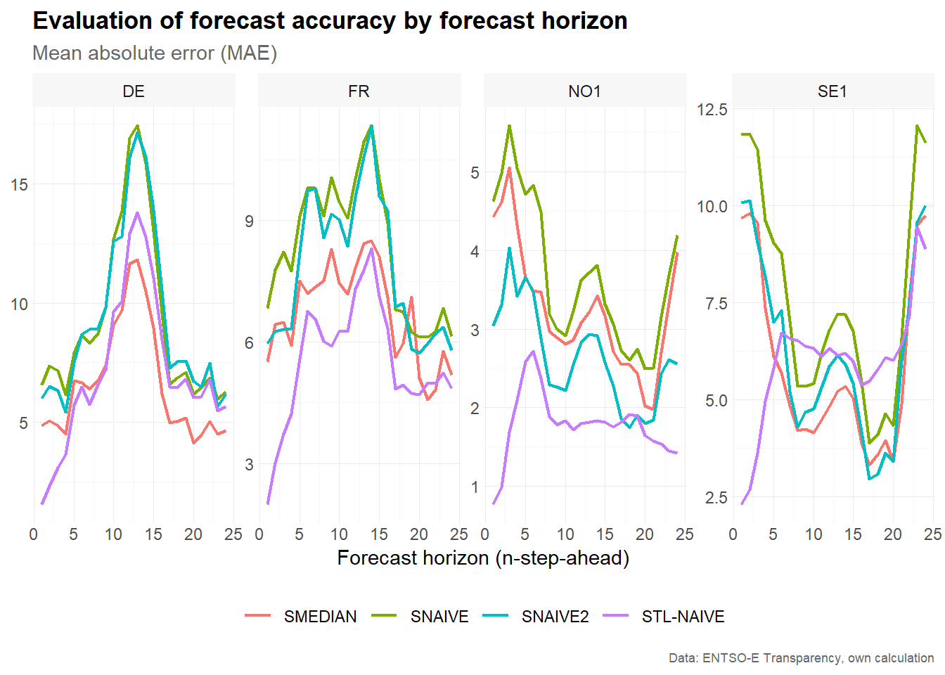
The resulting plot compares the mean absolute error across forecast horizons for each bidding zone and model. Increasing values indicate that forecasts become less accurate further into the forecast horizon. Differences between models show which benchmark performs best at different horizons.

Forecast accuracy by split

Accuracy by split is useful for identifying forecast origins where all models perform relatively well or poorly. This can reveal periods with unusual price behavior, such as strong volatility, negative prices or sudden price spikes.


# Estimate accuracy metrics by forecast horizon
accuracy_split <- make_accuracy(
  future_frame = future_frame,
  main_frame = main_frame,
  context = context,
  dimension = "split"
)

accuracy_split
#> # A tibble: 5,600 × 6
#>    bidding_zone model   dimension     n metric value
#>    <chr>        <chr>   <chr>     <int> <chr>  <dbl>
#>  1 DE           SMEDIAN split         1 MAE     2.80
#>  2 DE           SMEDIAN split         2 MAE     3.74
#>  3 DE           SMEDIAN split         3 MAE     2.70
#>  4 DE           SMEDIAN split         4 MAE     2.53
#>  5 DE           SMEDIAN split         5 MAE     4.54
#>  6 DE           SMEDIAN split         6 MAE     3.78
#>  7 DE           SMEDIAN split         7 MAE     4.38
#>  8 DE           SMEDIAN split         8 MAE     4.87
#>  9 DE           SMEDIAN split         9 MAE    11.5 
#> 10 DE           SMEDIAN split        10 MAE     5.02
#> # ℹ 5,590 more rows

# Visualize results
accuracy_split %>%
  filter(metric == "MAE") %>%
  plot_line(
    x = n,
    y = value,
    facet_var = bidding_zone,
    facet_nrow = 1,
    color = model,
    title = "Evaluation of forecast accuracy by split",
    subtitle = "Mean absolute error (MAE)",
    xlab = "Split",
    caption = "Data: ENTSO-E Transparency, own calculation"
    )

Plot accuracy by split

The resulting plot compares the mean absolute error across rolling-origin splits. Large error values for a particular split indicate that the corresponding 24-hour test window was difficult to forecast. Comparing models across splits helps assess whether forecast performance is stable over time.

Summary

This vignette demonstrated how to use tscv for time series cross-validation with a fixed window approach. The workflow consists of four main steps:

Prepare the data and define the column context.
Create fixed rolling-origin splits using make_split().
Estimate forecasting models separately for each time series and split.
Evaluate forecast accuracy by horizon and by split.

The fixed window approach is useful when the training sample should represent a recent period of constant length. This can be particularly helpful for time series such as electricity prices, where seasonal patterns, volatility and market conditions may change over time.

Alexander Häußer

Mai 2026