Tune hyperparameters of an Echo State Network (ESN) based on
time series cross-validation (i.e., rolling forecast). The input series is
split into n_split expanding-window train/test sets with test size
n_ahead. For each split and each hyperparameter combination
(alpha, rho, tau) an ESN is trained via train_esn() and
forecasts are generated via forecast_esn().
Arguments
- y
Numeric vector containing the response variable (no missing values).
- n_ahead
Integer value. The number of periods for forecasting (i.e. forecast horizon).
- n_split
Integer value. The number of rolling train/test splits.
- alpha
Numeric vector of candidate leakage rates. Smaller values produce slower reservoir state updates; larger values make the reservoir react more strongly to recent inputs.
- rho
Numeric vector of candidate spectral radii. This parameter scales the recurrent reservoir weights and affects reservoir memory and stability.
- tau
Numeric vector of candidate reservoir scaling values. Used to determine the reservoir size when
n_states = NULLintrain_esn().- min_train
Integer value. Minimum training sample size for the first split.
- ...
Further arguments passed to
train_esn()(exceptalpha,rho, andtau, which are set by the tuning grid).
Value
An object of class "tune_esn" (a list) with:
pars: Atibblewith one row per hyperparameter combination and split. Columns includealpha,rho,tau,split,train_start,train_end,test_start,test_end,mse,mae, andid.fcst: A numeric matrix of point forecasts withnrow(fcst) == nrow(pars)andncol(fcst) == n_ahead.actual: The original input seriesy(numeric vector), returned for convenience.
Details
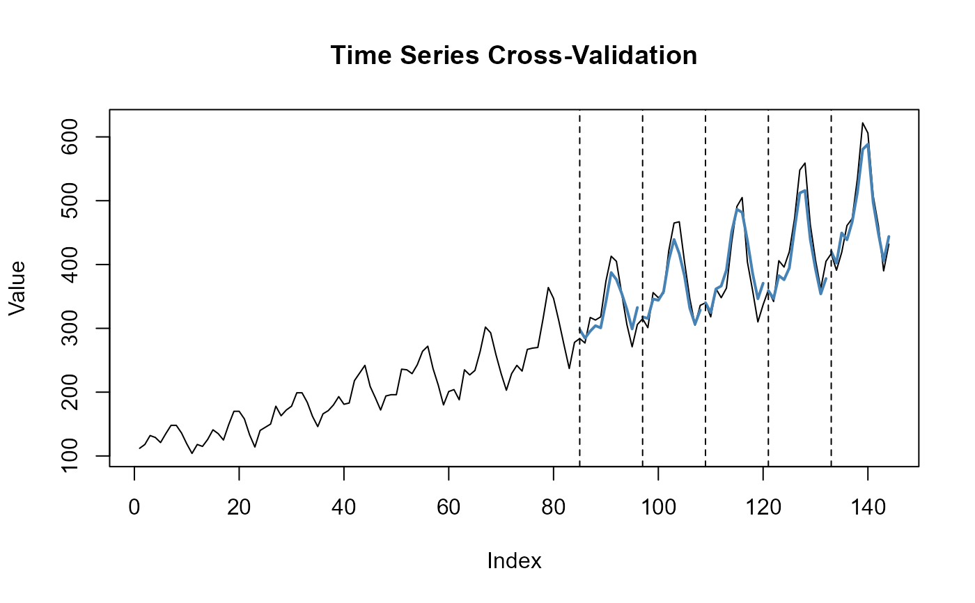
tune_esn() performs grid-based hyperparameter tuning using
expanding-window time series cross-validation. The tuning grid is formed
from all combinations of alpha, rho, and tau.
For each split, the model is trained on observations from the beginning
of the series up to the split-specific training endpoint and evaluated on
the following n_ahead observations.
For every candidate configuration and split, train_esn() is called
with the corresponding alpha, rho, and tau; all other
arguments supplied through ... are passed to train_esn().
Forecasts are generated with forecast_esn(), and the mean squared
error (mse) and mean absolute error (mae) are stored. The
accompanying summary() and plot() methods use these stored
errors to identify and display the best-performing hyperparameter
configuration.
Runtime increases approximately linearly with the number of grid combinations and the number of validation splits. Users should start with coarse grids and increase the grid resolution only where needed.
References
Häußer, A. (2026). Echo State Networks for Time Series Forecasting: Hyperparameter Sweep and Benchmarking. arXiv preprint arXiv:2602.03912, 2026. https://arxiv.org/abs/2602.03912
Jaeger, H. (2001). The “echo state” approach to analysing and training recurrent neural networks with an erratum note. Bonn, Germany: German National Research Center for Information Technology GMD Technical Report, 148(34):13.
Jaeger, H. (2002). Tutorial on training recurrent neural networks, covering BPPT, RTRL, EKF and the "echo state network" approach.
Lukosevicius, M. (2012). A practical guide to applying echo state networks. In Neural Networks: Tricks of the Trade: Second Edition, pages 659–686. Springer.
Lukosevicius, M. and Jaeger, H. (2009). Reservoir computing approaches to recurrent neural network training. Computer Science Review, 3(3):127–149.
See also
Other base functions:
forecast_esn(),
is.esn(),
is.forecast_esn(),
is.tune_esn(),
plot.esn(),
plot.forecast_esn(),
plot.tune_esn(),
print.esn(),
summary.esn(),
summary.tune_esn(),
train_esn()
Examples
xdata <- as.numeric(AirPassengers)
fit <- tune_esn(
  y = xdata,
  n_ahead = 12,
  n_split = 5,
  alpha = c(0.5, 1),
  rho   = c(1.0),
  tau   = c(0.4),
  inf_crit = "bic"
)
summary(fit)
#> # A tibble: 5 × 11
#>   alpha   rho   tau split train_start train_end test_start test_end   mse   mae
#>   <dbl> <dbl> <dbl> <int>       <int>     <int>      <int>    <int> <dbl> <dbl>
#> 1     1     1   0.4     1           1        84         85       96  471.  19.5
#> 2     1     1   0.4     2           1        96         97      108  376.  14.2
#> 3     1     1   0.4     3           1       108        109      120  526.  19.0
#> 4     1     1   0.4     4           1       120        121      132  547.  20.2
#> 5     1     1   0.4     5           1       132        133      144  396.  17.0
#> # ℹ 1 more variable: id <int>
plot(fit)